Project 5 / Face Detection with a Sliding Window
Introduction
This project is an example of the sliding window classification model in computer vision. This classification model is very prevalent and accurate at object detection, namely face recognition. In this project, the implementation is based on the 2005 paper by Dalal and Triggs, which uses a histogram of gradients to represent faces. Given a training set of known faces and non-faces, a HoG can be generated for each positive and negative datapoint and used to train a classifier. After the classifier is trained, the general idea is to take a sliding window across some unseen image or scene and let the classifier determine if the given window in the scene is a face or not. For some positive match, if the confidence of the classifier is above some set threshold, then the image pipeline would identify that as a face.
Feature Extraction, Feature Representation, and Classifier Training
The first 3 parts of the project involved generating positive and negative features for a classifier algorithm and then training the algorithm. The positive features were created from known ground truths while negative features were randomly sampled from images that were known not to have faces. In this pipeline, the features were histograms of gradients. After the features were extracted, an simple vector machine (linear classifier) was trained with the positive and negative labeled data. As a sanity check, the SVM was tested on the training data, and as expected, performed well.
Initial classifier performance on train data:
  accuracy:            0.999
  true  positive rate: 0.398
  false positive rate: 0.000
  true  negative rate: 0.601
  false negative rate: 0.000
Single-Scale Detection
The first facial detector implemented was a single-scale detector, which did not resize the image in any way. All the single-scale detector did was use a sliding window on each test image, generate a HoG for the sliding window, and query the SVM to see whether the bounding window was a face.
Average Results
Average precision: 0.314

True positives: 175
False positives: 392.33
False negatives: 336

Total time: 108.848 s
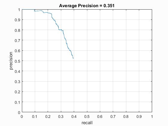
These results were used as a baseline for the future changes and tweaks of the detection pipeline. As a note, the cell size was 6, the lambda value was 0.0001 and the confidence threshold was 0.75. These values may become relevant later.
Multi-Scale Detection
Multi-scale detection fixes one of the biggest problems in single-scale detection, which is that faces can be of different scale in an image. Multi-scale runs the same sliding window detector algorithm at different scales of the image so that faces of different scale can still be found.
Averages
Average precision: 0.858

True positives: 460
False positives: 483.33
False negatives: 51

Total time: 195.121 s
Raw Results
Run 1Average precision: 0.873
True positives: 467
False positives: 431
False negatives: 44
Total time: 196.815 s
Average precision: 0.853

True positives: 459
False positives: 363
False negatives: 52

Total time: 195.234 s
Average precision: 0.847

True positives: 454
False positives: 521
False negatives: 57

Total time: 193.313 s
Analysis
Empirically, the most noticeable improvement was in the average precision, which rose from an average of 0.351 to an average of 0.874. Additionally, the average false negatives fell to double digits as the algorithm was able to identify different-scaled faces.
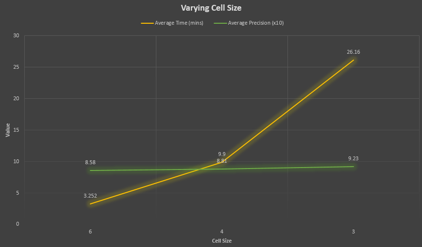
Varying Cell Size
In an attempt to further improve the precision and results of the facial detection, the cell size was decreased to 4 pixels and 3 pixels respectively. In theory, by reducing the values cell size values, the average precision should increase because the algorithm will using a more granular step for each image.
Cell Size of 4
Averages
Average precision: 0.881

True positives: 480.67
False positives: 306.67
False negatives: 30.33

Total time: 594.173 s
Raw Results
Run 1Average precision: 0.865
True positives: 485
False positives: 223
False negatives: 26
Total time: 601.425 s
Average precision: 0.887

True positives: 474
False positives: 444
False negatives: 37

Total time: 588.612 s
Average precision: 0.891

True positives: 483
False positives: 253
False negatives: 28

Total time: 592.481 s
Cell Size of 3
Averages
Average precision: 0.923

True positives: 485
False positives: 261
False negatives: 26

Total time: 601.623 s
Raw Results
Run 1Average precision: 0.923
True positives: 485
False positives: 141
False negatives: 26
Total time: 1569.855 s
Average precision: 0.934

True positives: 489
False positives: 386
False negatives: 22

Total time: 1602.842 s
Average precision: 0.913

True positives: 481
False positives: 256
False negatives: 30

Total time: 1688.123 s
Analysis
It is clear that lowering the cell size improves performance and granularity of the pipeline. As expected, a cell size of 3 performed the best, with an average precision of 0.923 and lows in both false positives and false negatives. However, there is a large time tradeoff when using such a granular cell size, which is time. The time for the 3 cell size pipeline takes nearly 30 minutes, while in comparison, the 6 cell size pipeline takes around 3 minutes. Given that tradeoff, however, the improvement in both the false positives and false negatives can be desirable when time is not an issue.
Varying Positive Match Threshold
The multi-scale detection's improvement over single-scale detection was very significant, and varying the cell sizes further tuned the results to be slightly more accurate. However, one of the glaring issues was the large amount of false positives, so in order to attempt to reduce the number of false positives, the confidence threshold for a positive match was varied.
Baseline Results

|
Threshold: 0.75

True positives: 467
False positives: 431
False negatives: 44
Experiment Results
Threshold: 0.5

True positives: 478
False positives: 787
False negatives: 33
Threshold: 0.75

True positives: 467
False positives: 431
False negatives: 44
Threshold: 0.80

True positives: 452
False positives: 344
False negatives: 59
Threshold: 0.85

True positives: 469
False positives: 388
False negatives: 42
Threshold: 0.90

True positives: 470
False positives: 589
False negatives: 41
Analysis
Varying the confidence interval threshold did not really improve the false positives, but there was a sweet spot for true positives and false positives around 0.85 as the threshold. The false positive non-improvement was likely due to the classifier being very confident on the false positive matches. As a result, there was not much improvement from before in that area.
Optimal Results
|
Threshold: 0.85

True positives: 452
False positives: 344
False negatives: 59
Note: The confidence level was tested on a cell size of 6, but the best result was then generated using a cell size of 3 for practical time reasons.
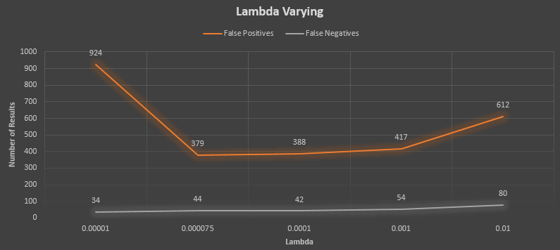
Varying SVM Lambda
Because changing the confidence threshold did not seem to really lower the false positive values, the SVM lambda value was tuned instead to see if there were better results. Perhaps the learning algorithm was not classifying the information with the correct parameters.
Baseline Results
|
|
Threshold: 0.0001

True positives: 469
False positives: 388
False negatives: 42
Experiment Results
Lambda: 0.00001

True positives: 477
False positives: 924
False negatives: 34
Lambda: 0.000075

True positives: 467
False positives: 379
False negatives: 44
Lambda: 0.0001

True positives: 469
False positives: 388
False negatives: 42
Lambda: 0.001

True positives: 457
False positives: 417
False negatives: 54
Lambda: 0.01

True positives: 431
False positives: 612
False negatives: 80
Analysis
Again, there seemed to be very little improvement from the baseline, but arguably the best performing lambda value was the same as the best performing value from the previous project (0.000075). This value was chosen as the default for the best results.
Optimal Results
|
Lambda: 0.000075

True positives: 469
False positives: 187
False negatives: 42
Note: The confidence level was tested on a cell size of 6, but the best result was then generated using a cell size of 3 for practical time reasons.
Best Results
These were the best results, using the best parameters found in each experiment. The parameters of note were lambda value of 0.000075, threshold of 0.85, and cell size of 3 pixels.
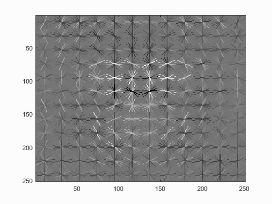
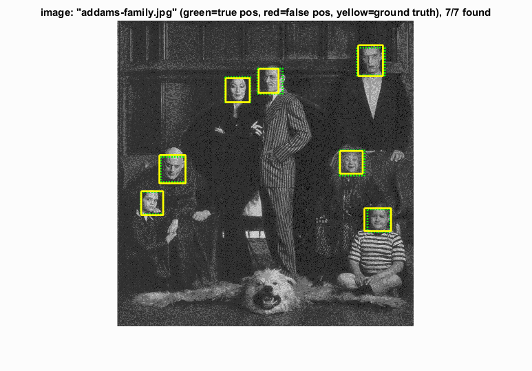
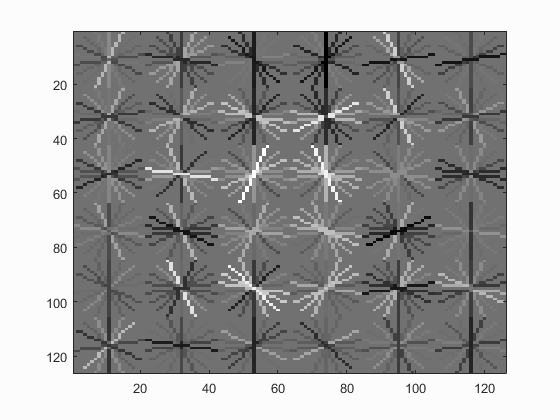
Histogram of Gradients.
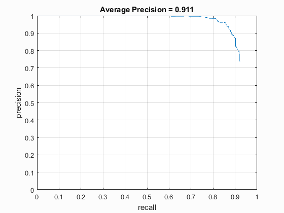
Precision graph.
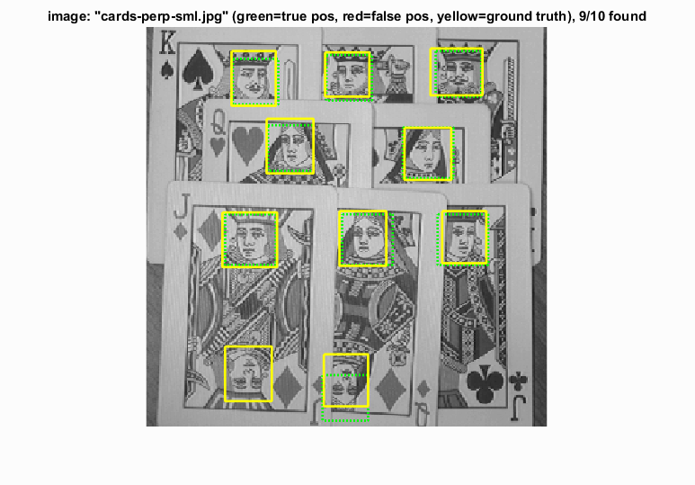
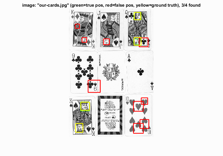
Cards Perp: A strong showing from the algorithm!
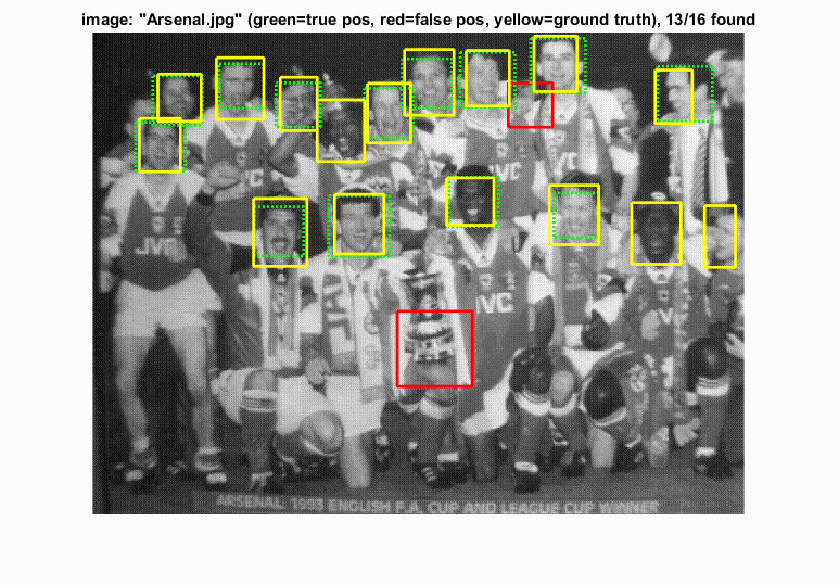
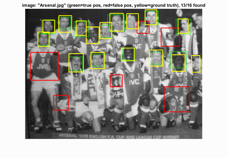
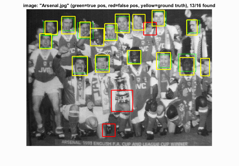
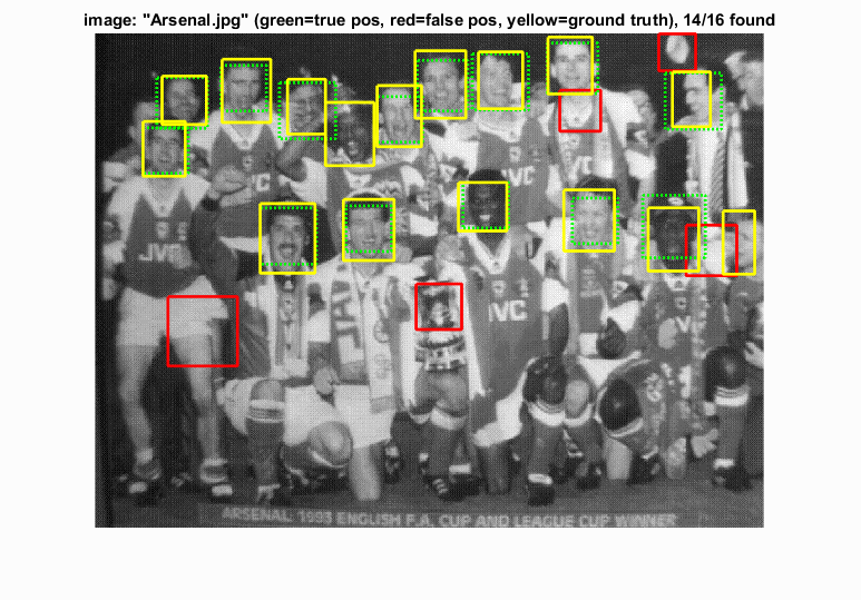
Arsenal: One of the most difficult images in the testing set that performed relatively well, despite the many false positives.
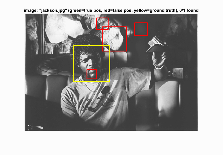
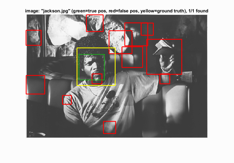
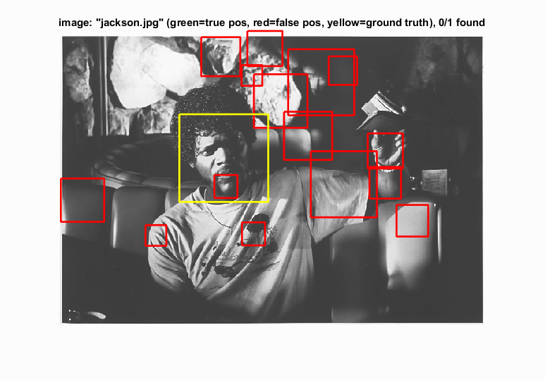
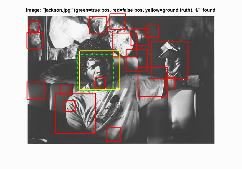
Jackson: Arguably one of the most difficult images in the testing set, with tough lighting for the algorithm to deal with.
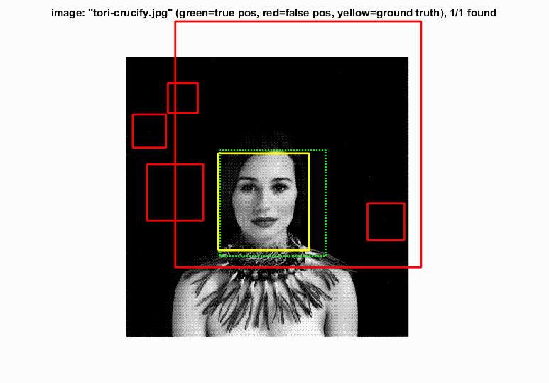
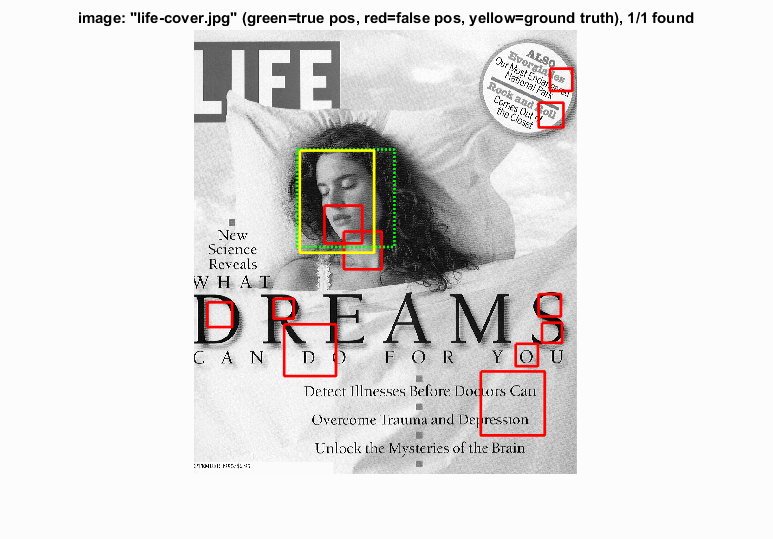
Additional Results
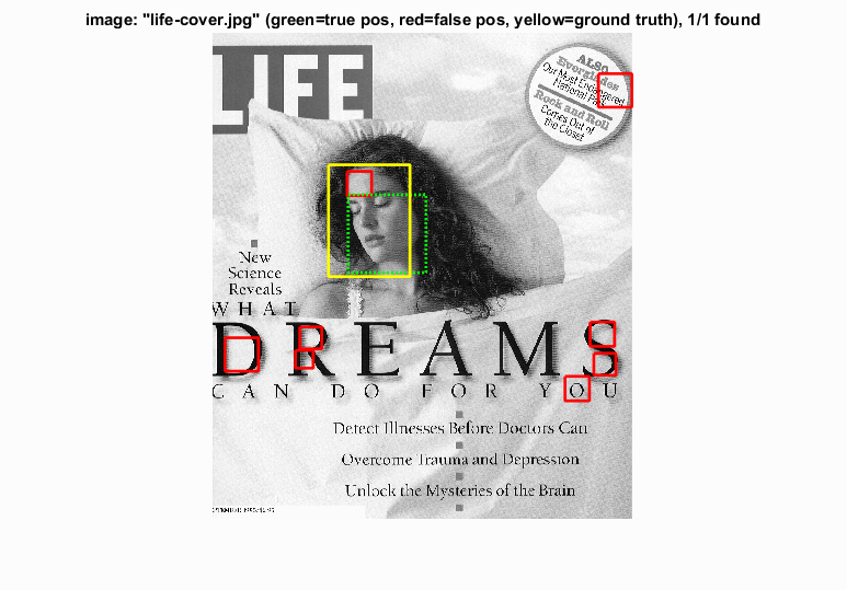
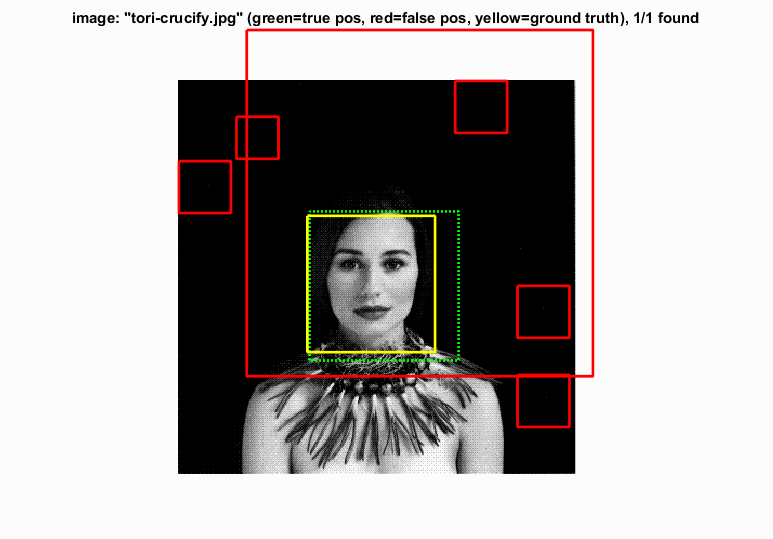
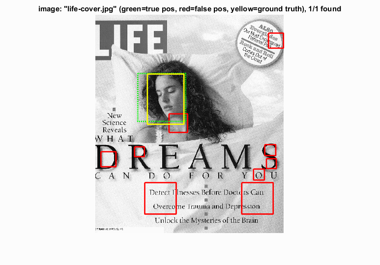
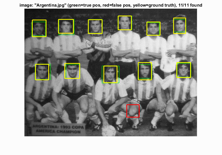
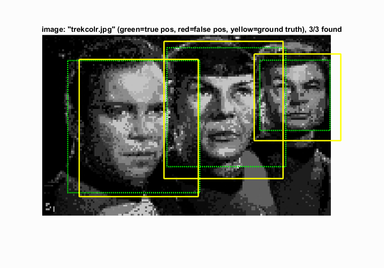
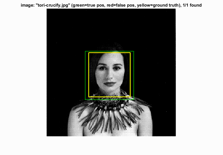
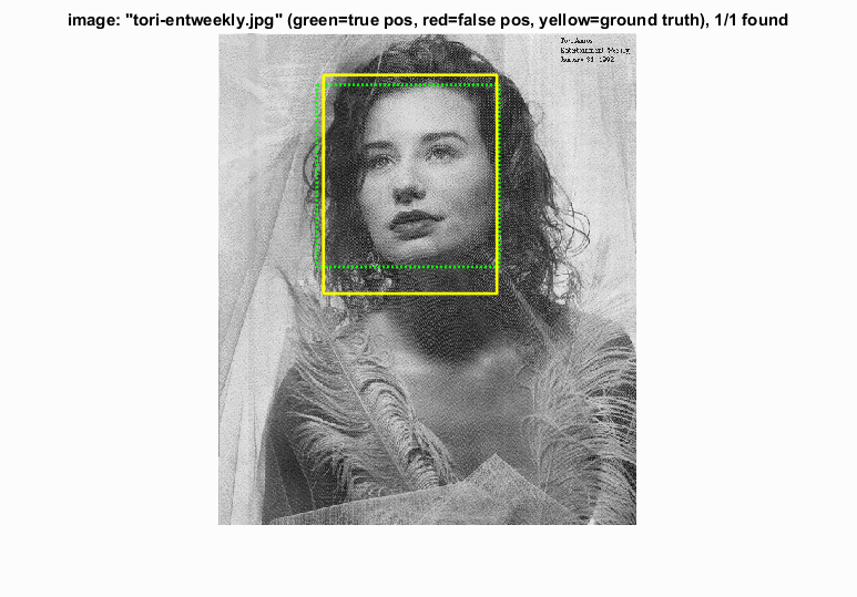
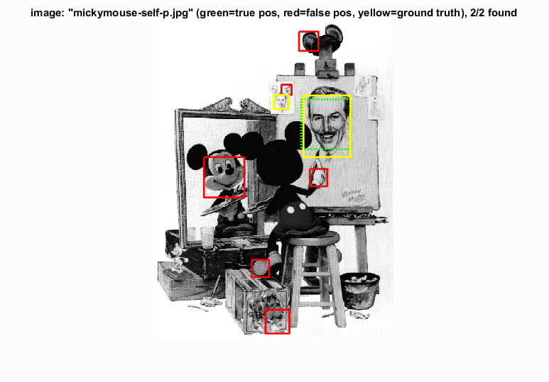
Good performing ones on top and troublesome results on bottom.
|

|