Project 5 / Face Detection with a Sliding Window
This goal of this project is to create a sliding window, multiscale face detector. We will use SIFT-like HoG features on patches, slide the patches along the images, and use SVM or other classifiers to classify the images. We will do this for multiple scales and return the bounding boxes of potential matches. Overlapping bounding boxes will be removed yeilding the final result.
STEP 1: get_positive_features.m and get_random_negative_features.m
When implmenting get_positive_features.m I first read in the image, make sure it is grayscale, then resize it to the size of the desired template size (36x36 pixels). I then found the hog features with vl_hog(). The resulting feature is 1116 dimensions. For get_random_negative_features, I randomly took patches of images at random scales and found their HoG features. The number of patches I sampled from each image was proportional to the size of the image. I collected 10,000 negative examples.
STEP 2: Train Classifier
For traning the classifier, I first used linear SVM, with vl_svmtrain(). I used a lambda value of 1.e-7.
STEP 3: run_detector.m
For run_detector.m I first perform downsampling to scale the image down. I repeatedly scaled the image down by a 90% 20 times or until the image was too small to extract the hog features. Once the image was scaled down I found the hog features, then used a sliding window to take patches of the hog features which were of the correct size to yield the right number of features. I used a step size of 6 pixels. I then ran the feature through the classifier and found the confidence value. If the confidence was higher than a threshold (for SVM, I used -0.1), then I saved the bounding box for that feature and the confidence as well. Finally, after performing this operation on the different scales, I used non maximum supression to find non-overlapping bounding boxes with the highest confidence. These were the positive labeled faces.
RESULTS
With the pipeline outlined above, I was able to achieve an average precision of 0.876. This is using a threshold for the SVM of -0.1. Below are the graphs for the results.
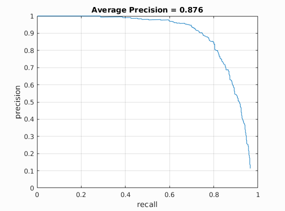
Average Precision.
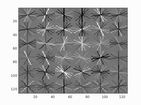
HoG Template.
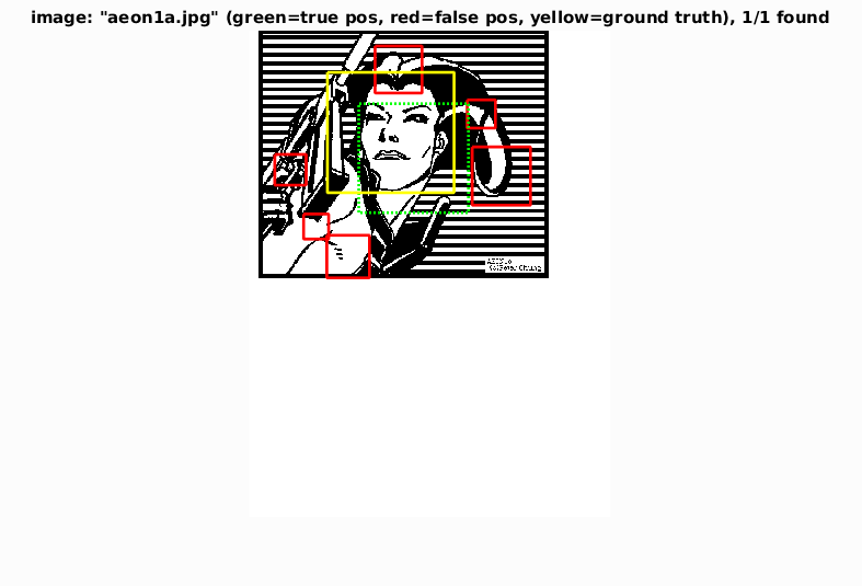
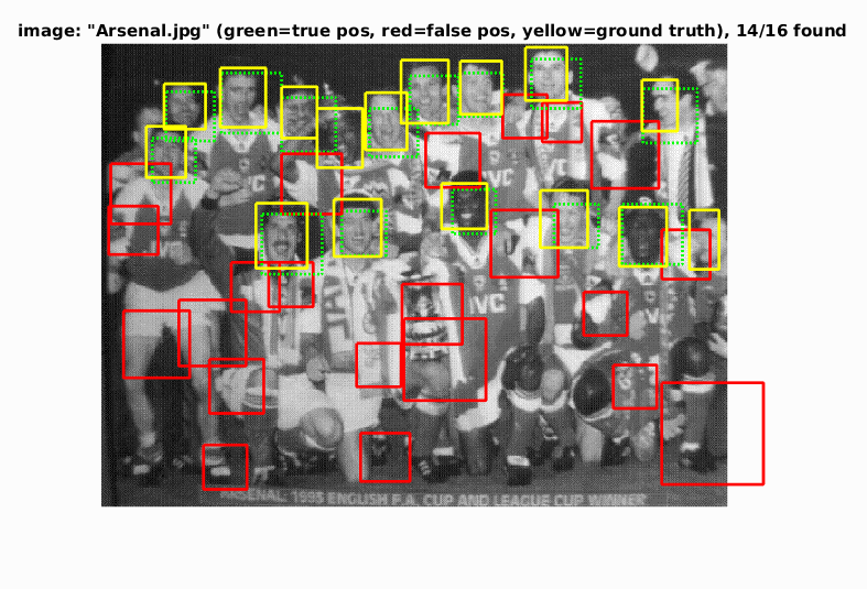
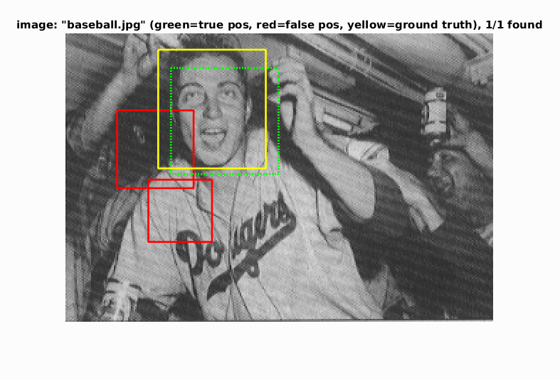
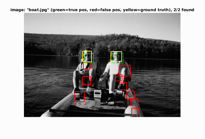
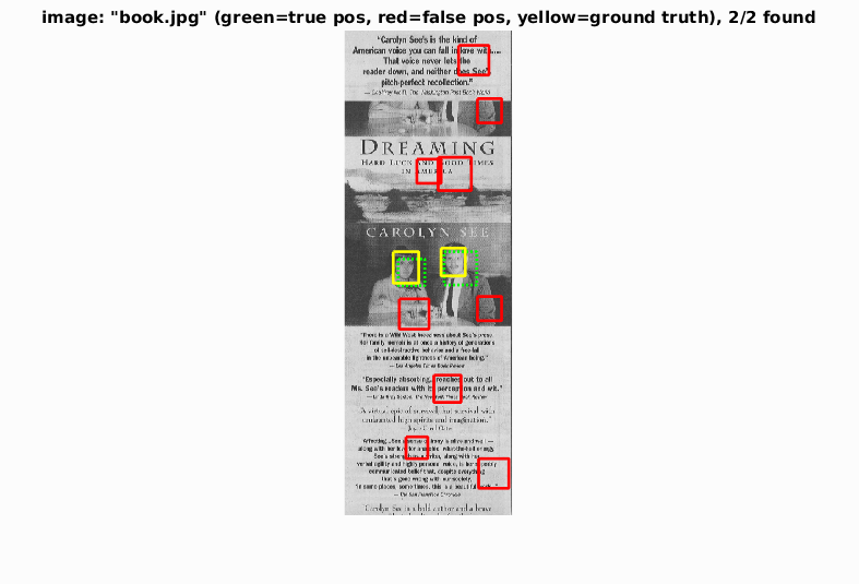
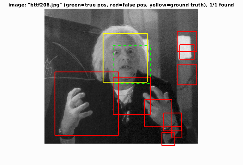
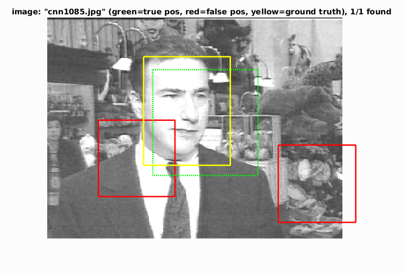
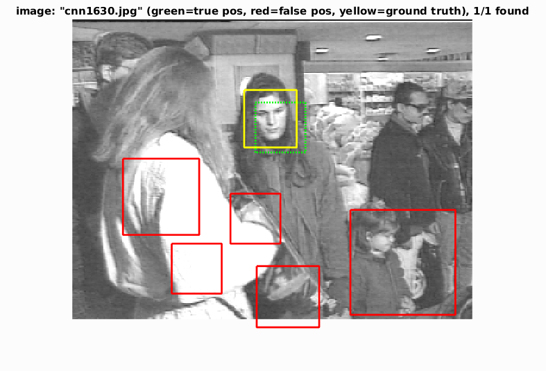
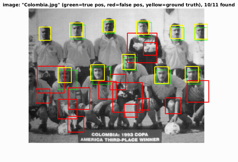
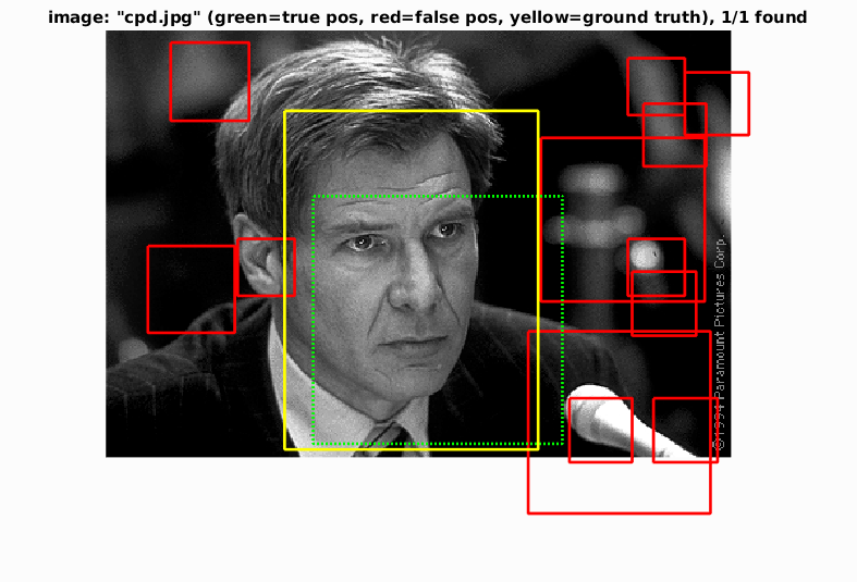
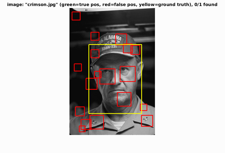
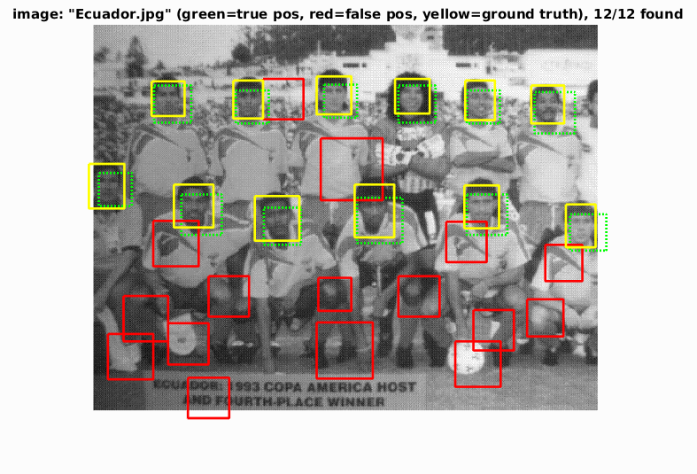
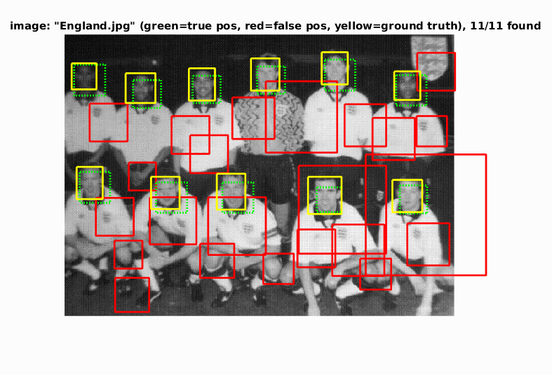
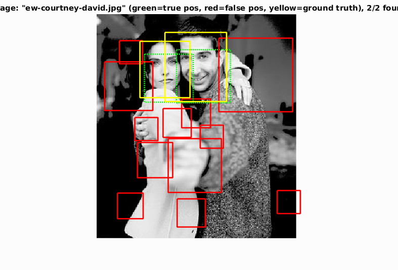
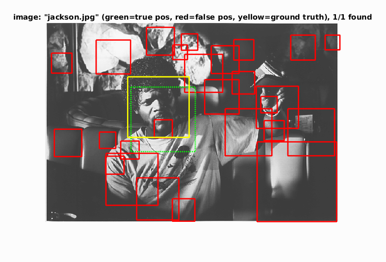
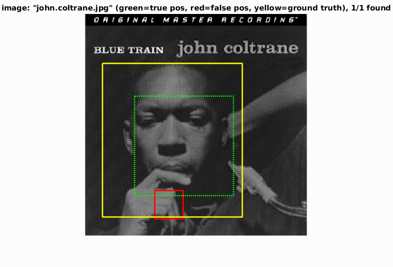
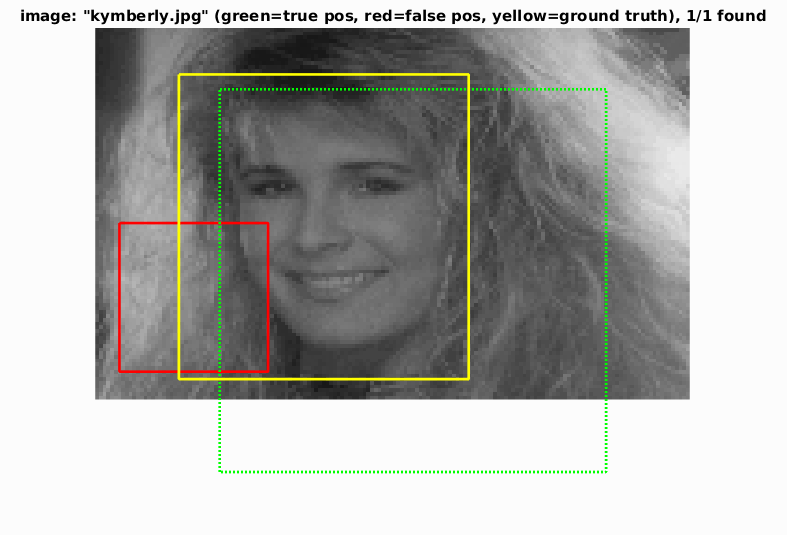
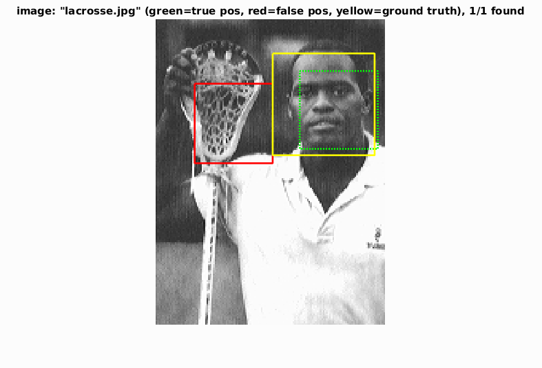
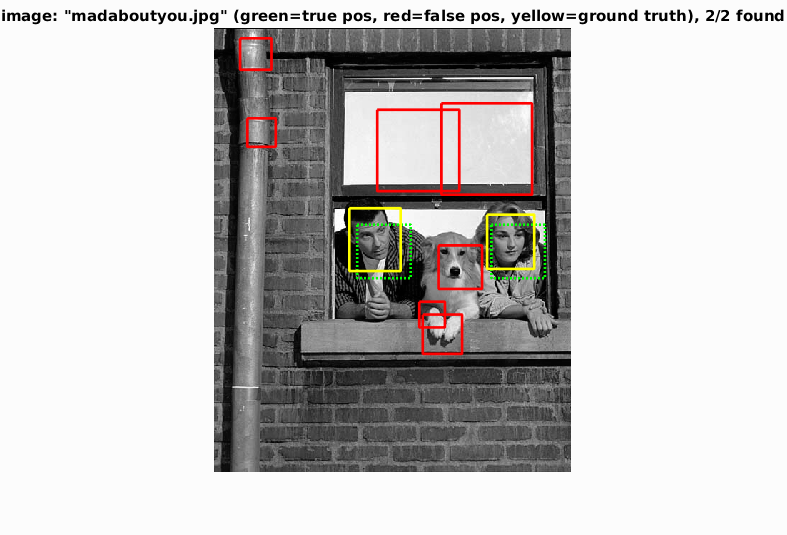
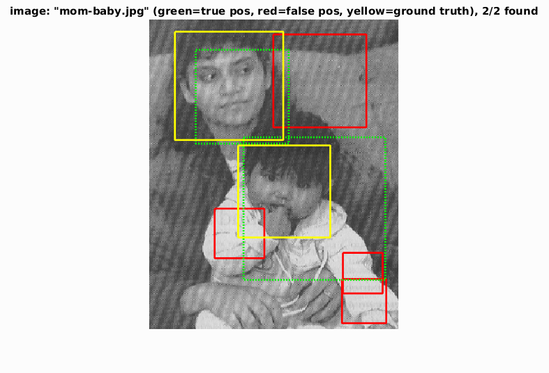
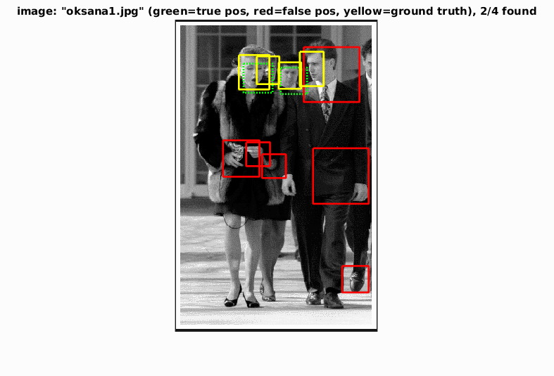
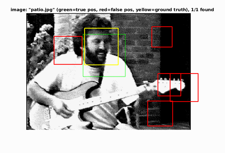
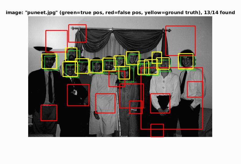
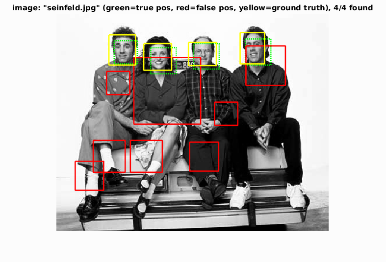
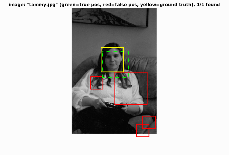
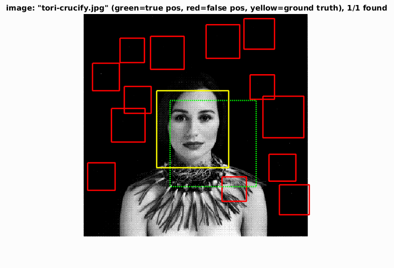
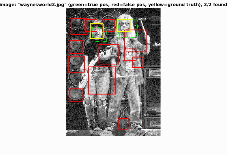
Using this low threshold gives a higher average precision, but returns too many false positives, yielding results like this:
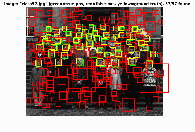
Too many false positives.
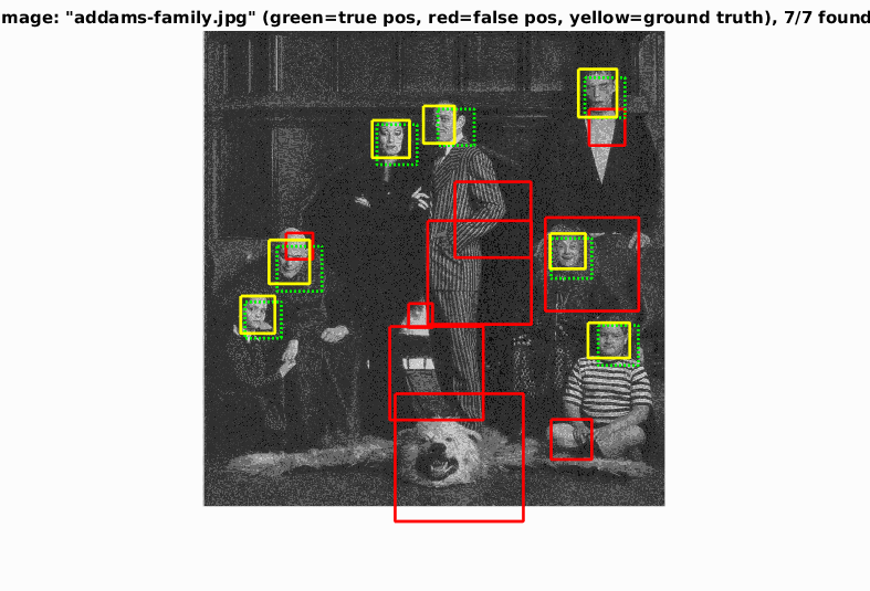
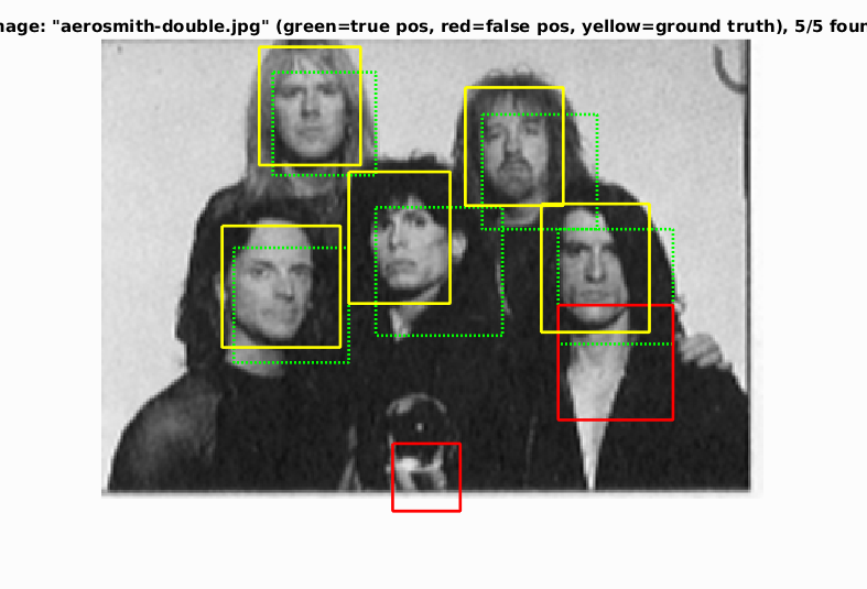
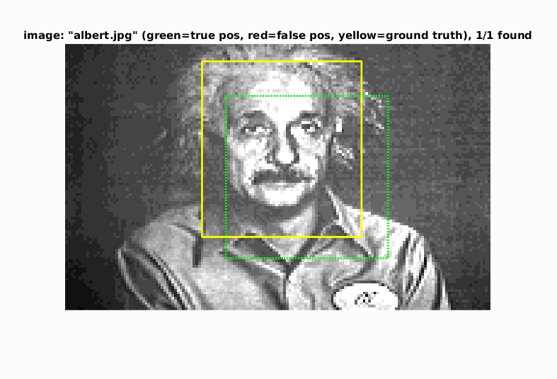
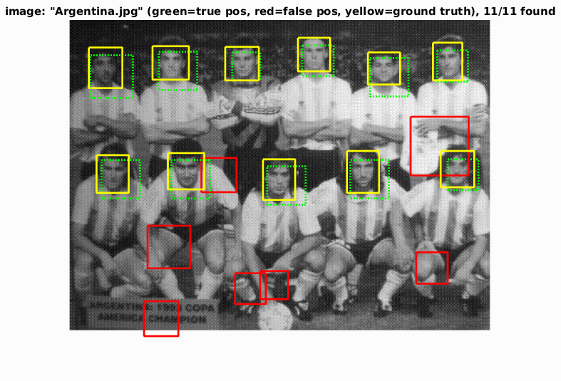
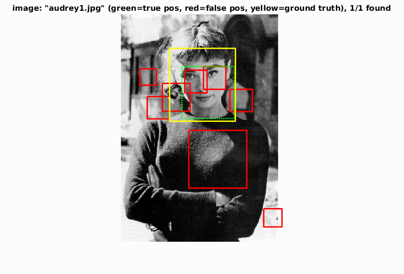
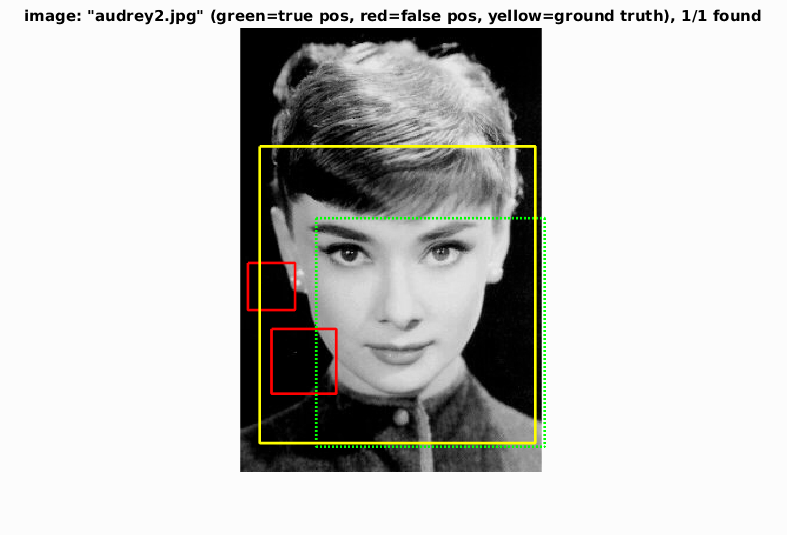
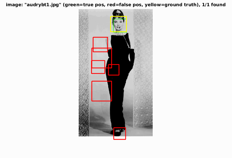
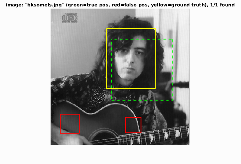
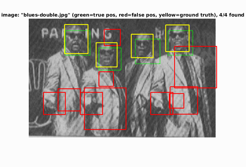
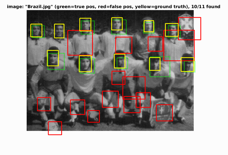
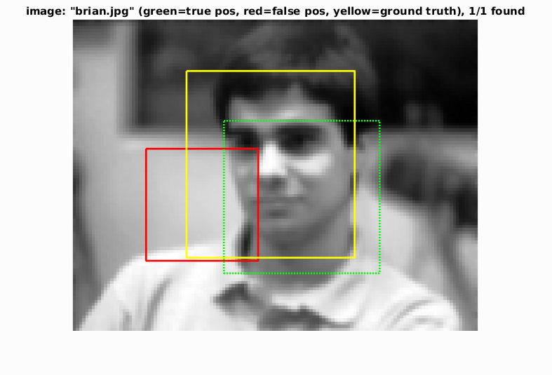
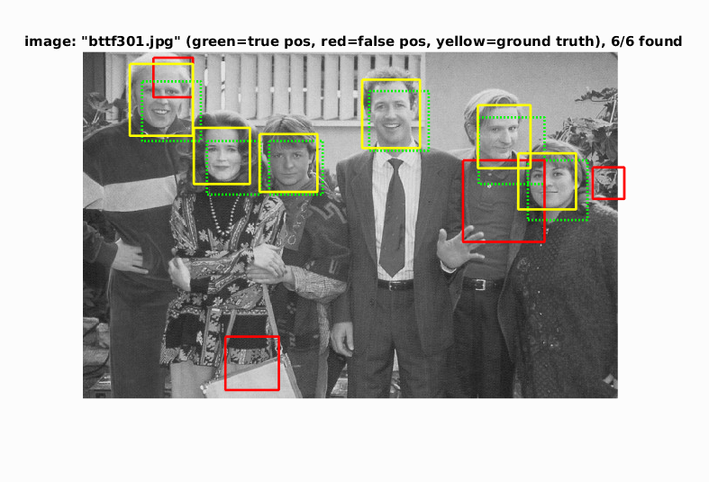
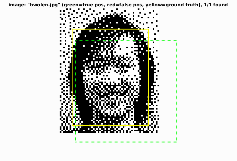
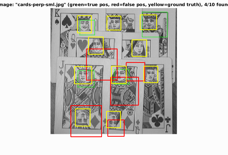
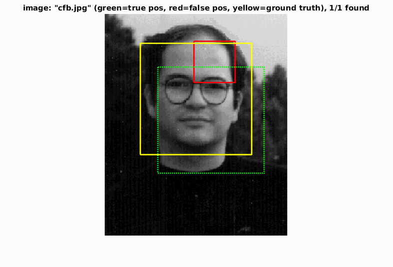
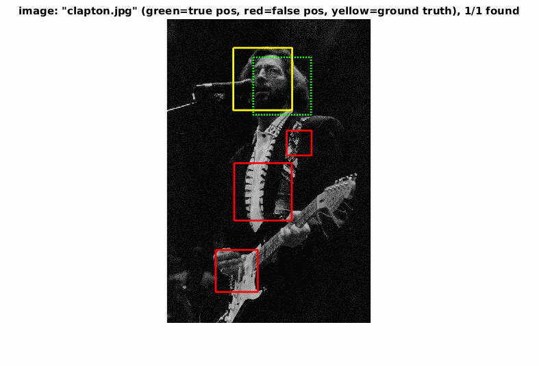
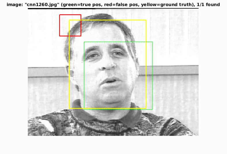
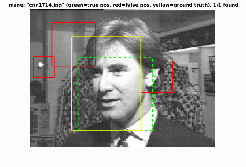
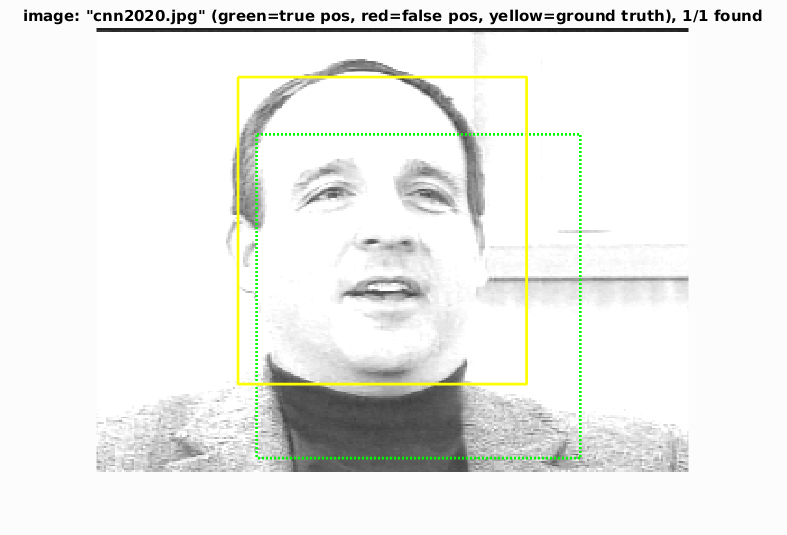
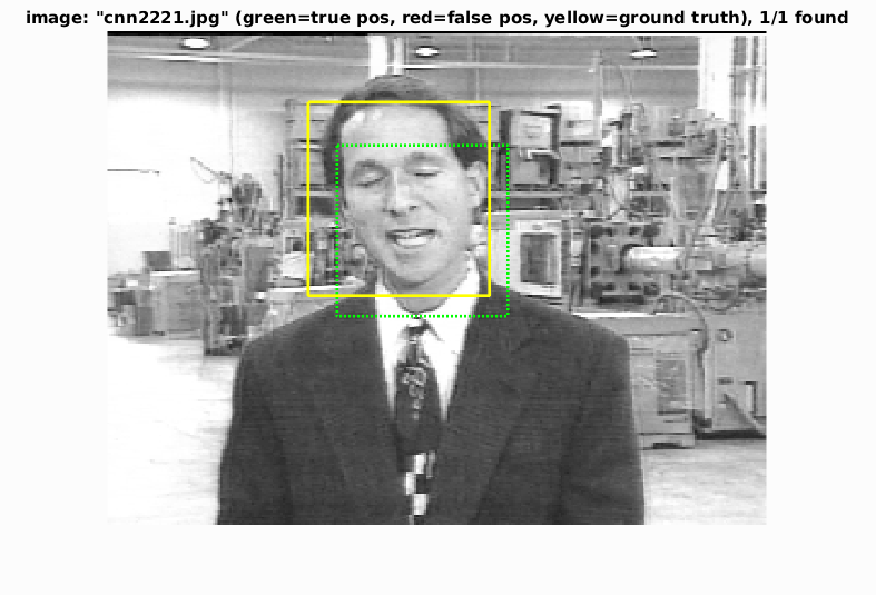
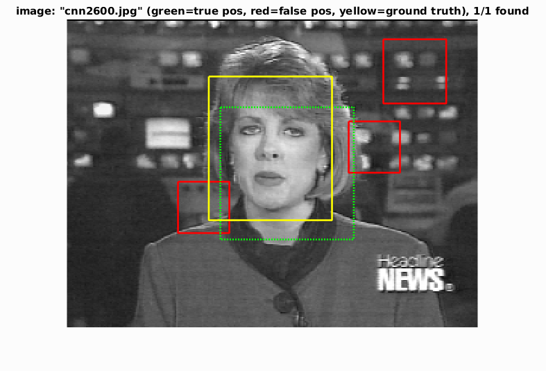
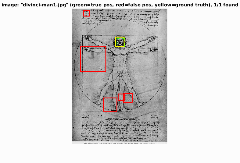
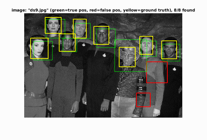
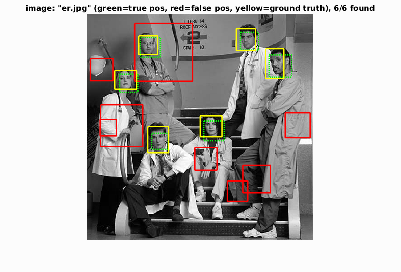
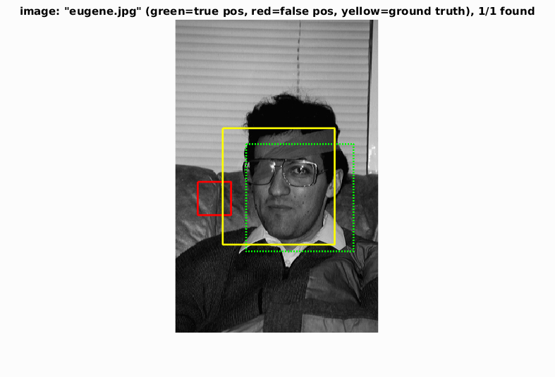
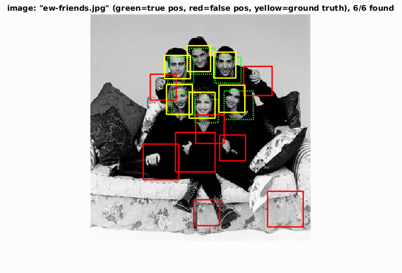
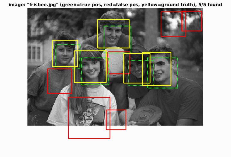
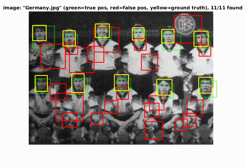
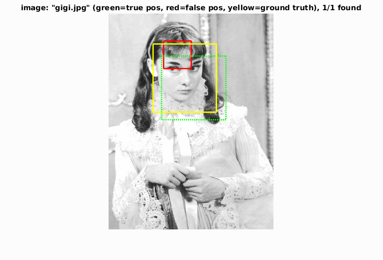
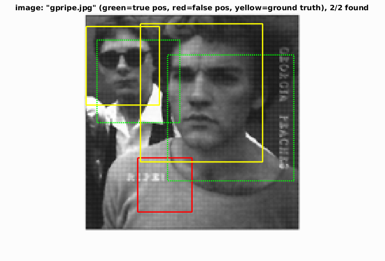
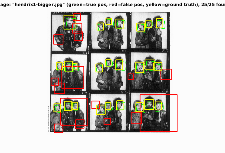
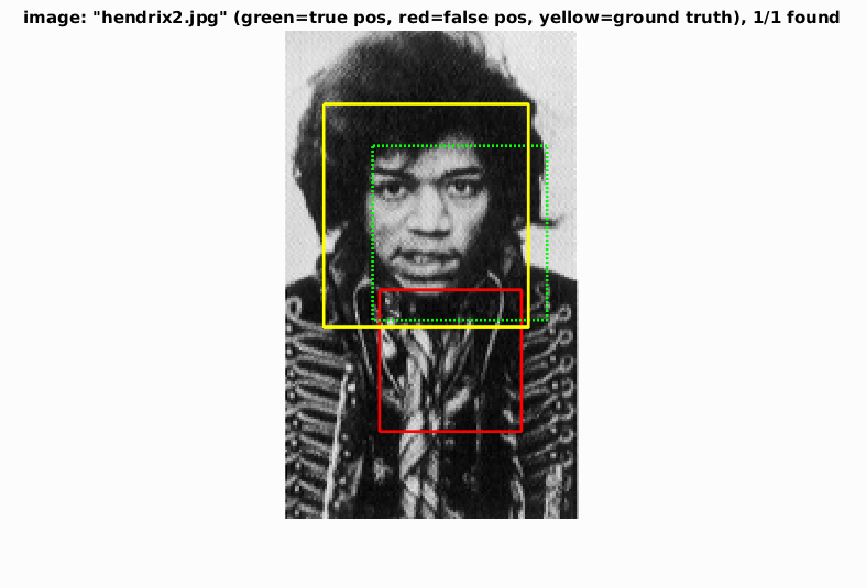
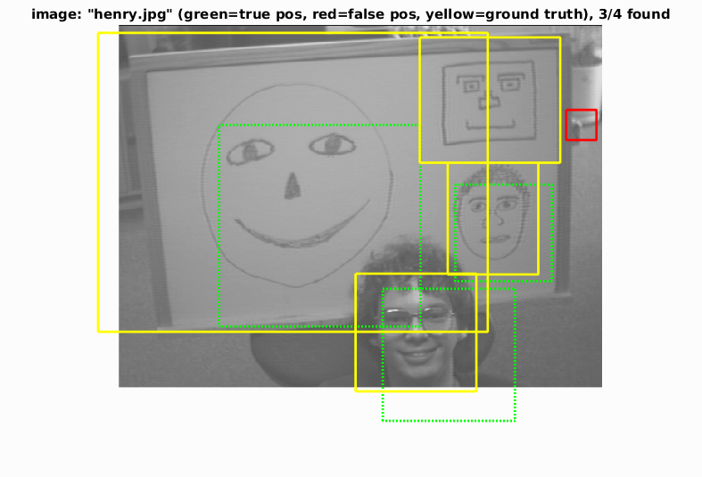
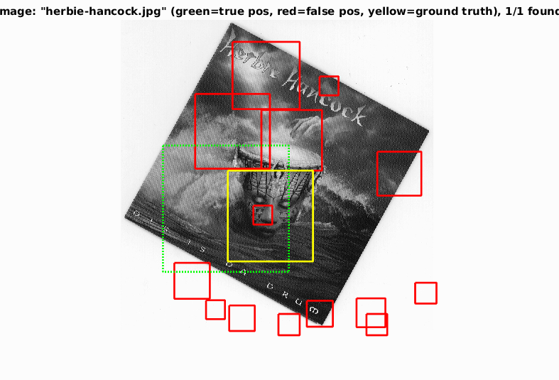
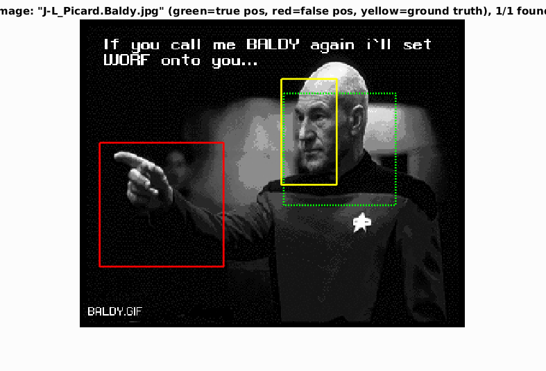
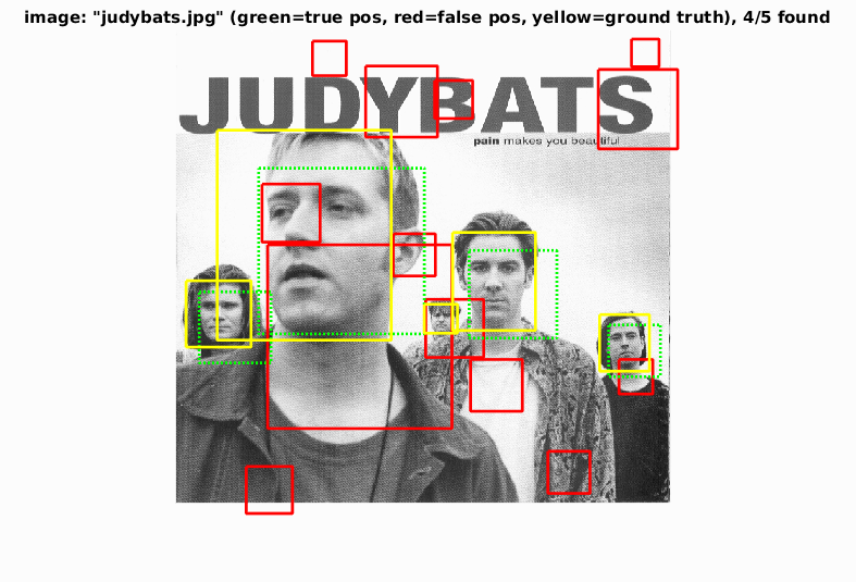
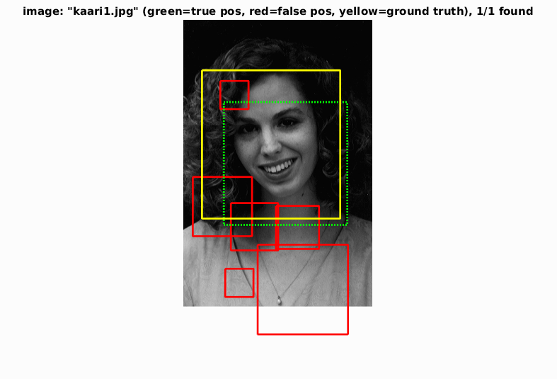
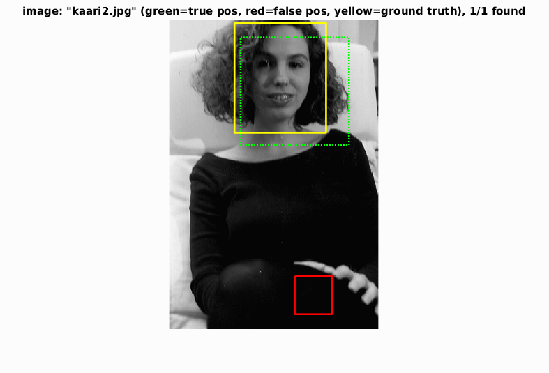
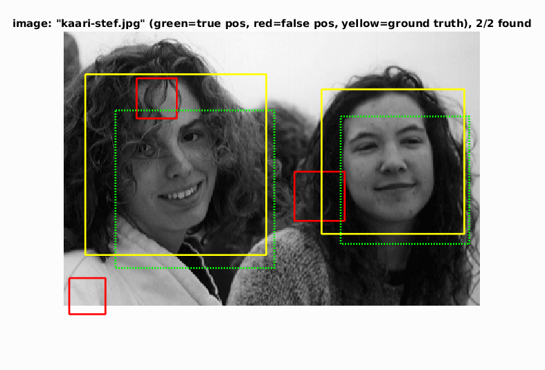
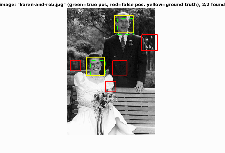
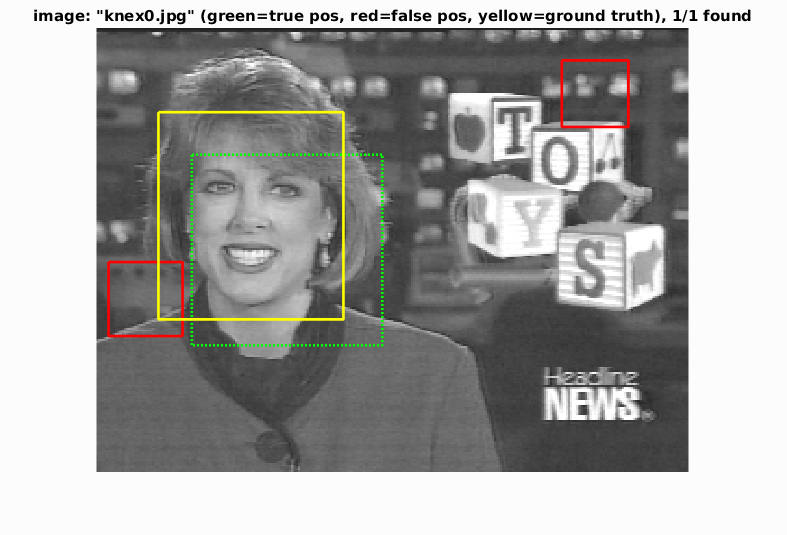
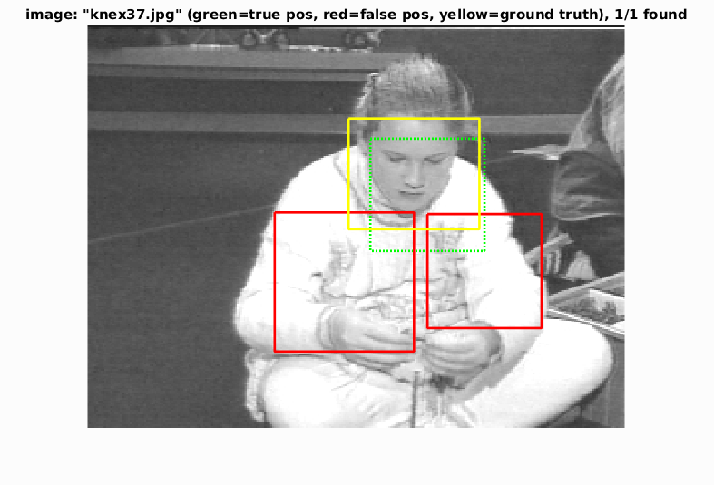
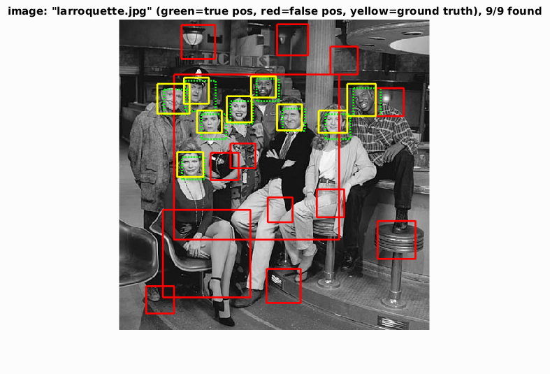
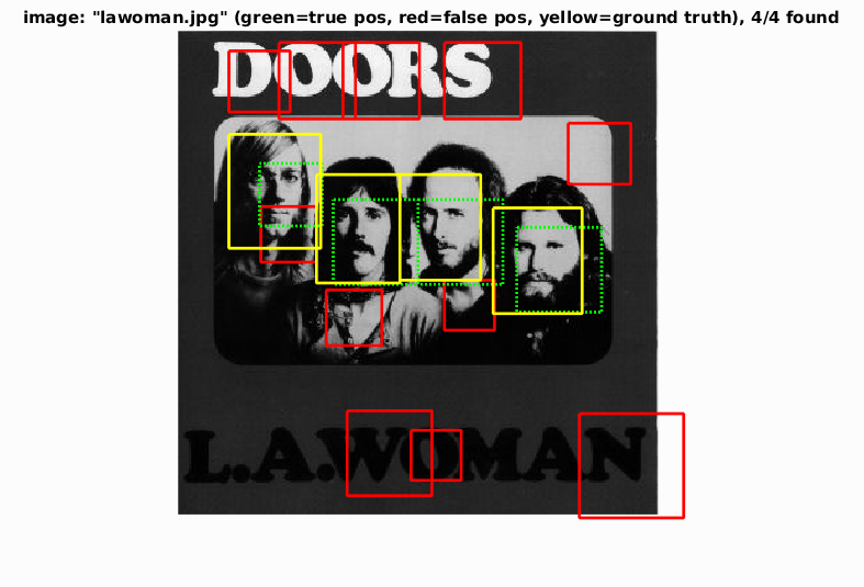
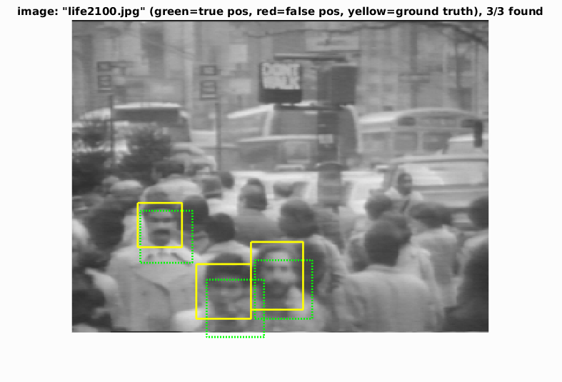
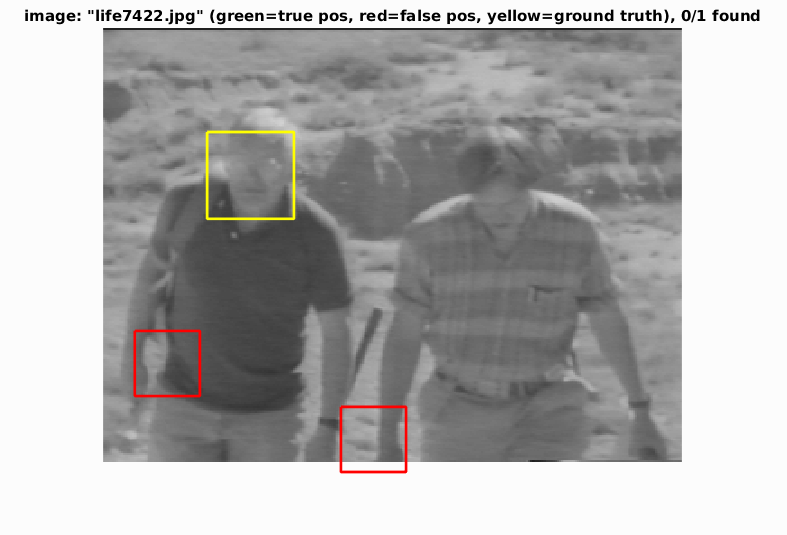
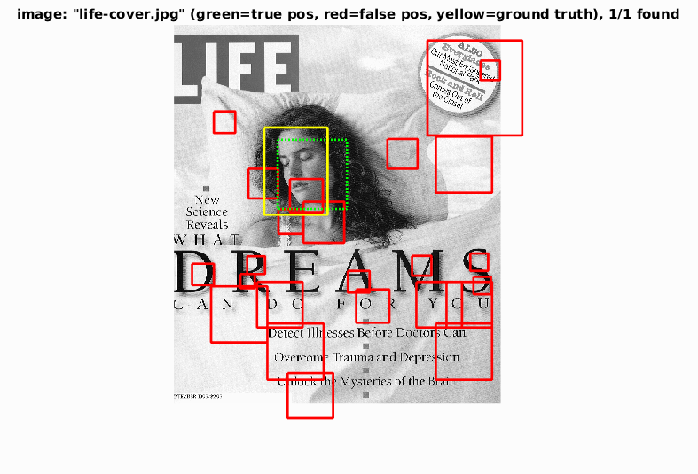
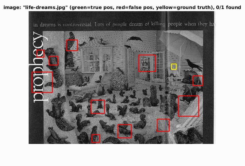
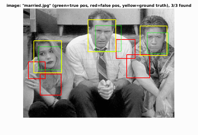
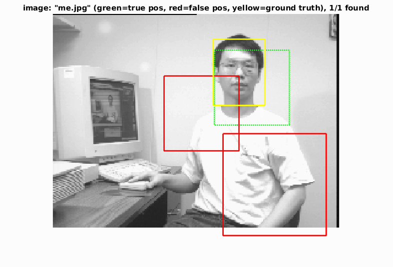
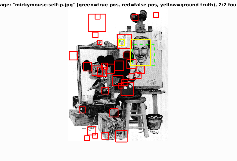
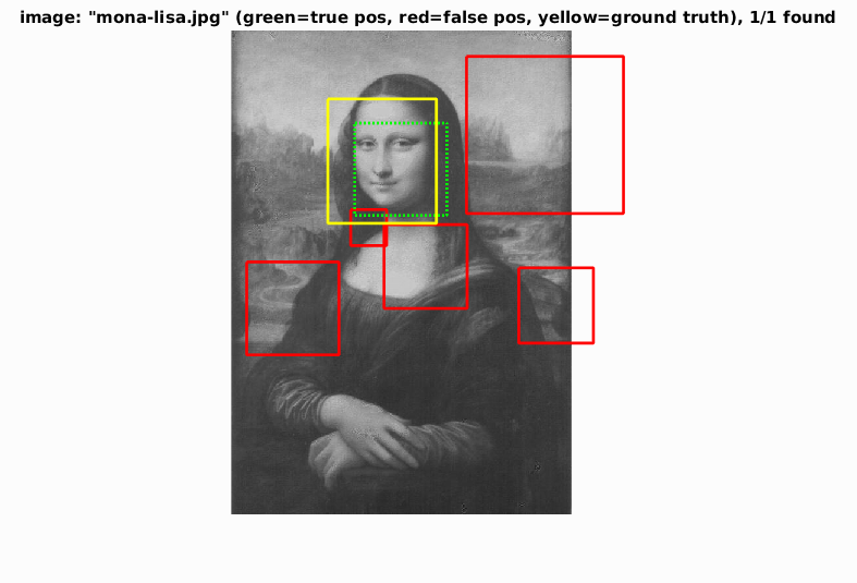
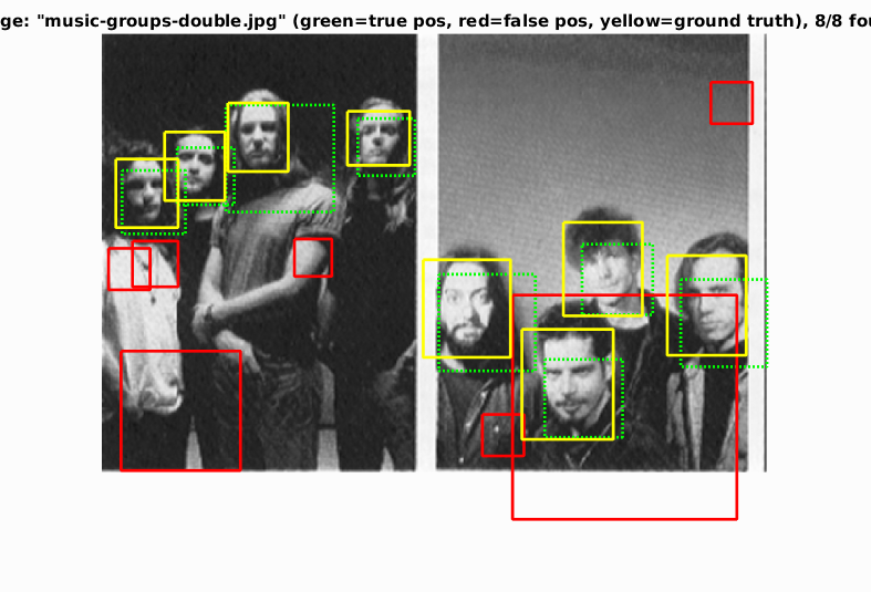
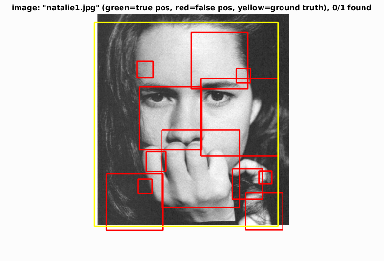
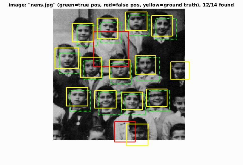
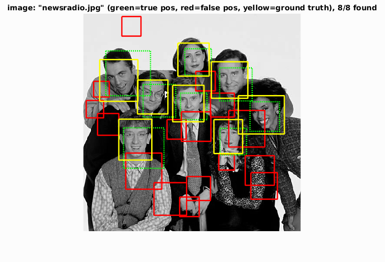
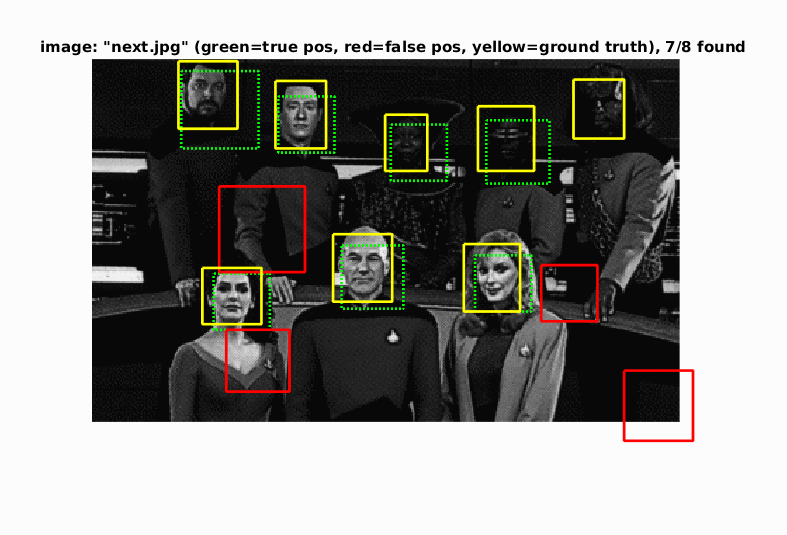
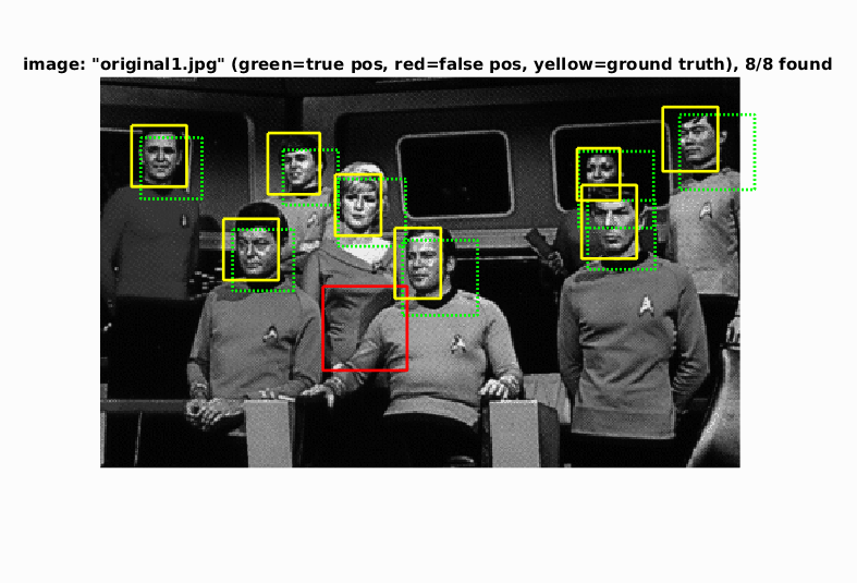
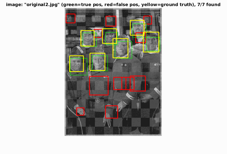
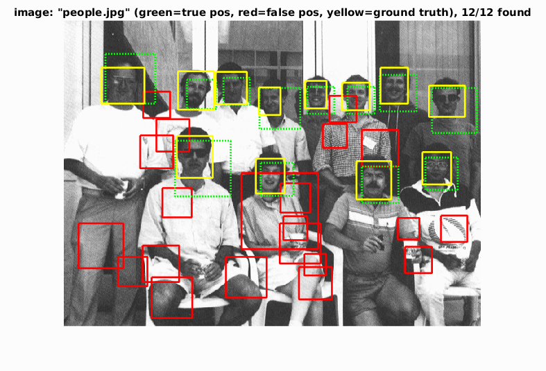
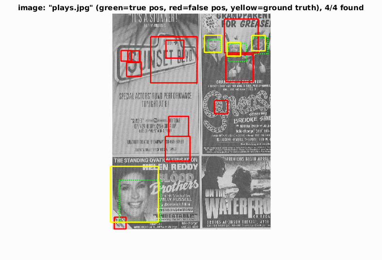
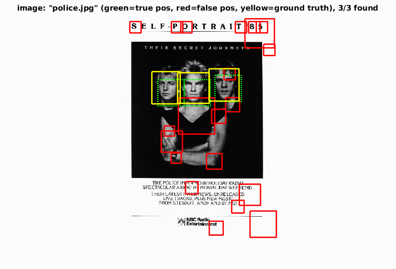
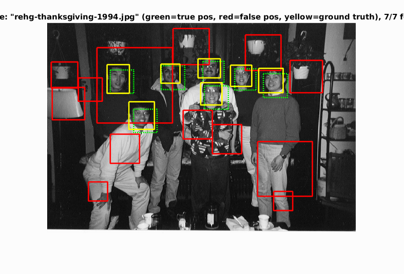
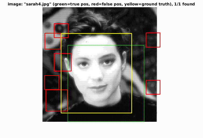
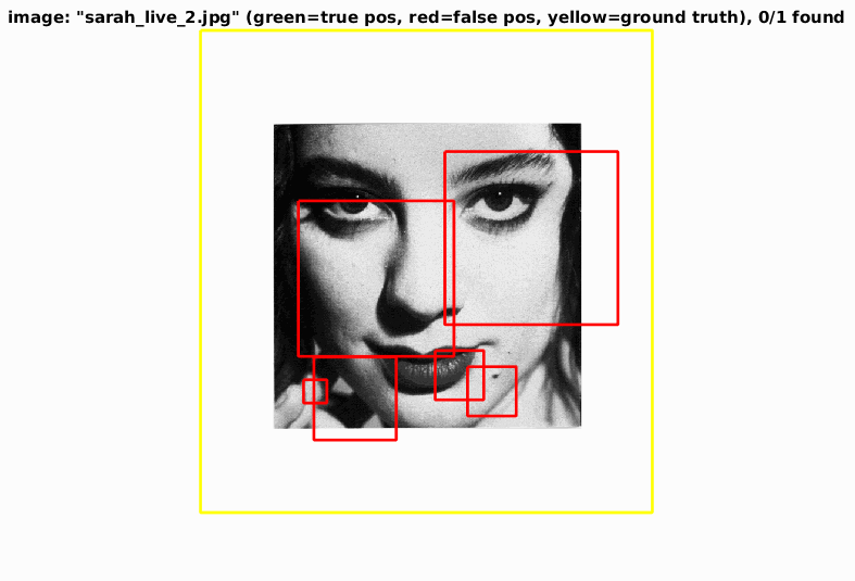
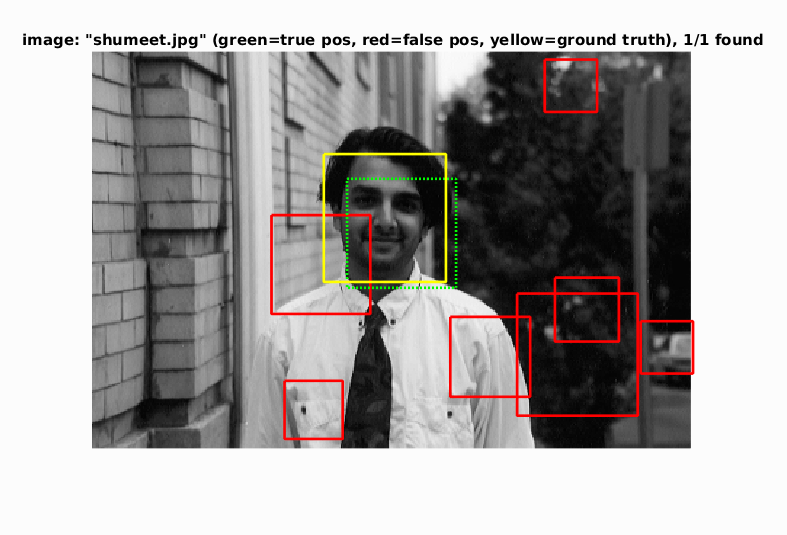
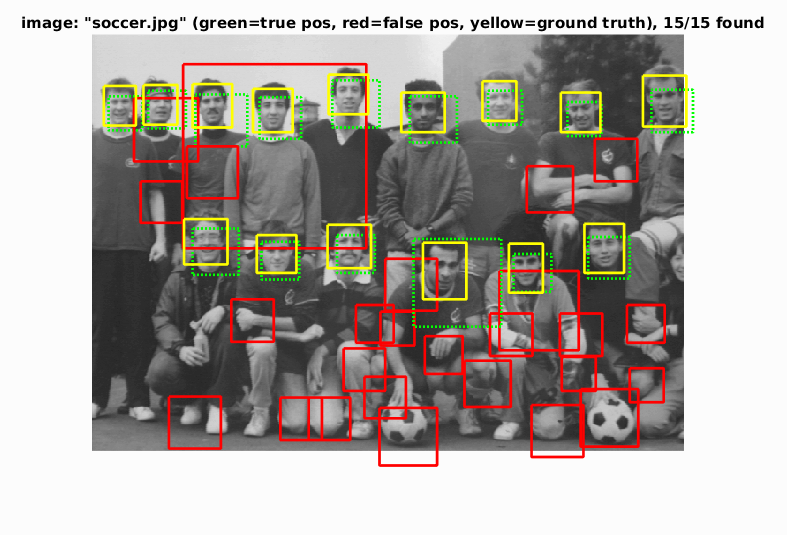
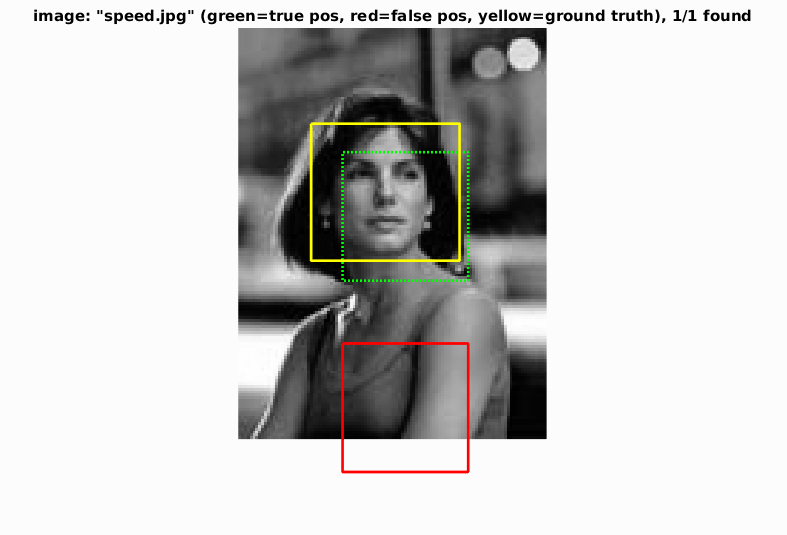
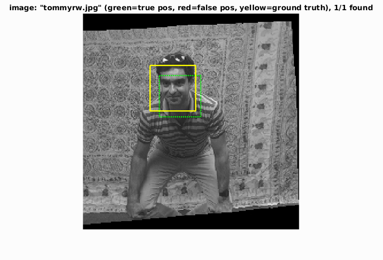
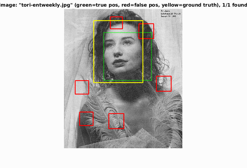
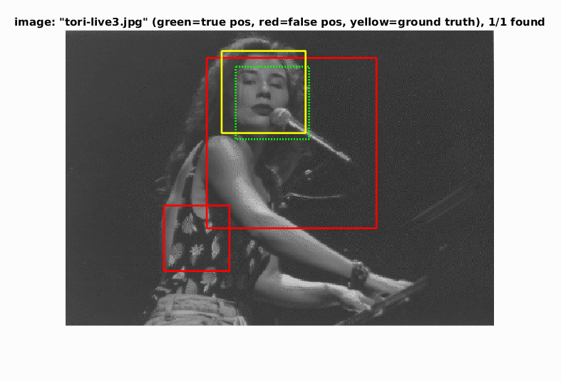
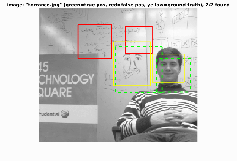
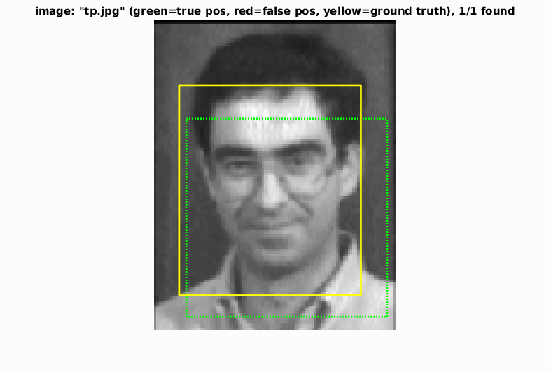
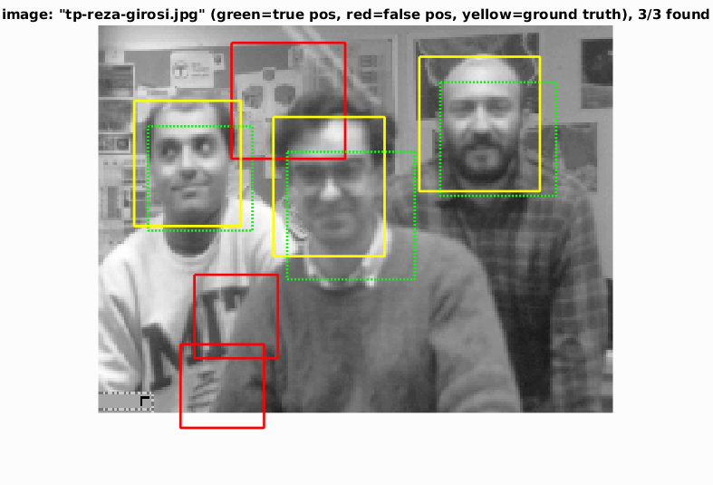
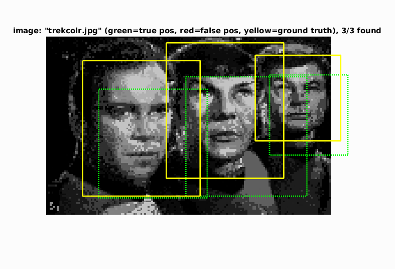
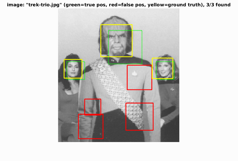
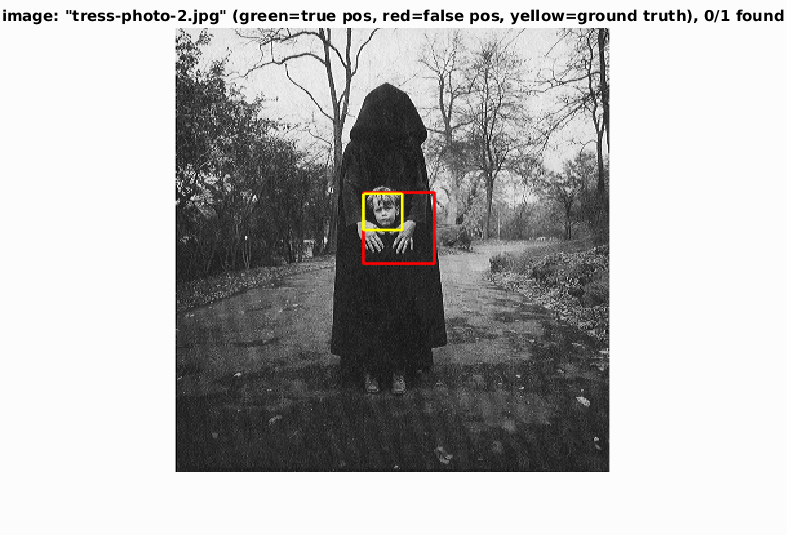
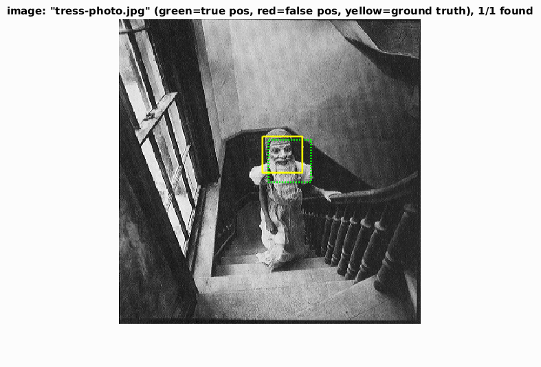
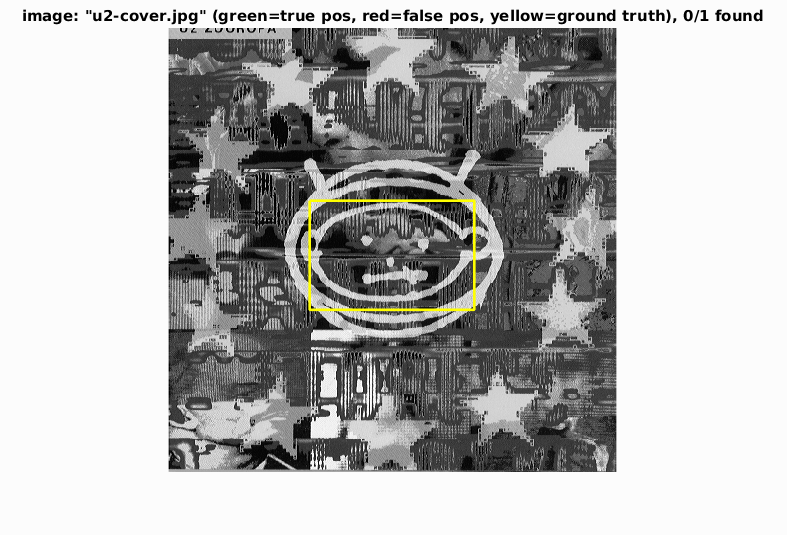
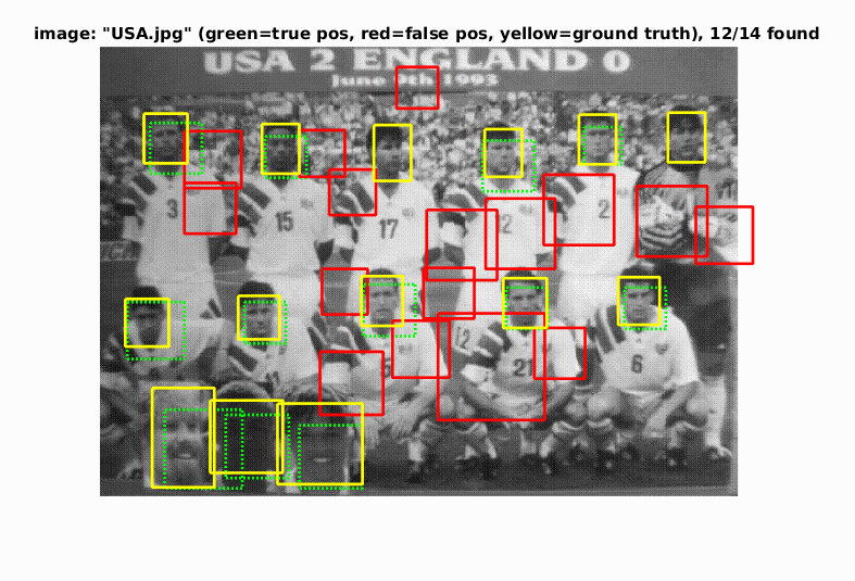
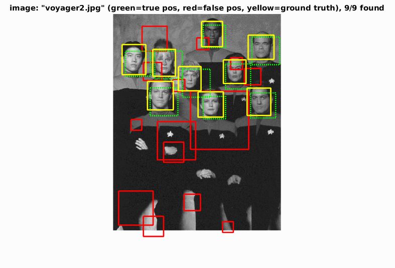
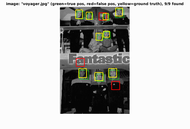
To reduce the false positive rate, I increased the threshold to 0.8. This resulted in a lower average precision of 0.871, with fewer false positives. Below are the results of the test images.
All results
|
EXTRA 1: Using other positive training data
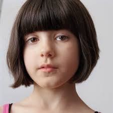
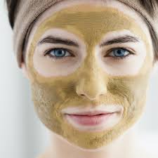
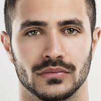
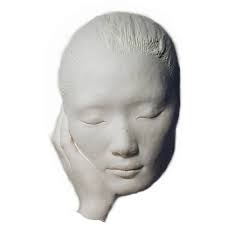
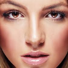
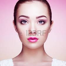
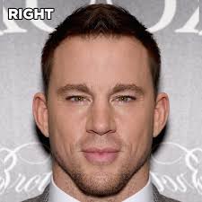
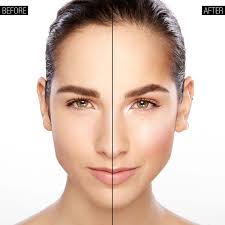
I found more positive face images by searching on google images and downloading the thumbnails. I tried to curate the search to return clear, head-on, square images containing human faces. I collected 731 images in this way. The search process was not perfect, but here are some examples of images I retrieved:


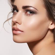
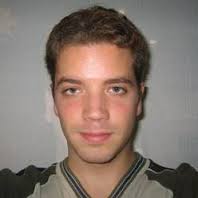

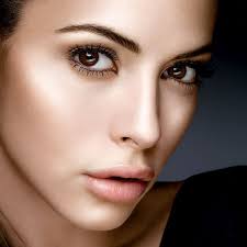
|
I scaled the images down to 36x36 and converted to greyscale, then incorporated these images into Caltech training dataset, yeilding a total of 6713+731=7444 positive images. I then ran the entire pipeline, hoping that the performance would improve. using a low threshold for the confidence of -0.1, I got an average precision of 0.653. This was lower than without using the additional images. This is probably due to the fact that the images I added were not very close to the test set. Specifically, there may have been too many side views of faces, which can be seen from the difference in the HoG template, which is less symmetric. This highlights the importance of carefully choosing good data.
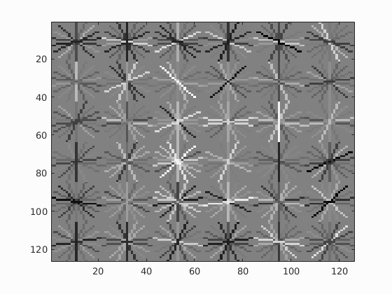
HoG template using extra images from google.
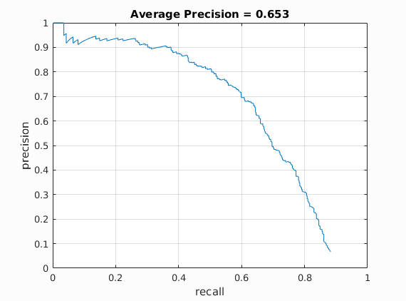
Average precision using extra images from google.
EXTRA 2: Using a Random Forest classifier
I tried using MATLAB's built in random forest classifier (fitcenemble) for the classification. This yielded worse results (AP 0.863). Below is the precision vs recall graph. The implmentation was considerably slower than linear SVM.
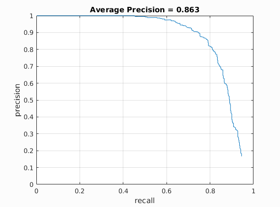
Average precision using random forests.
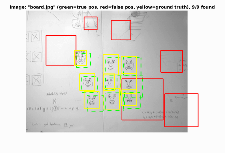
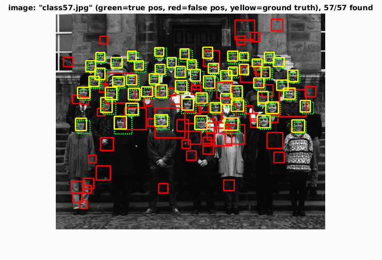
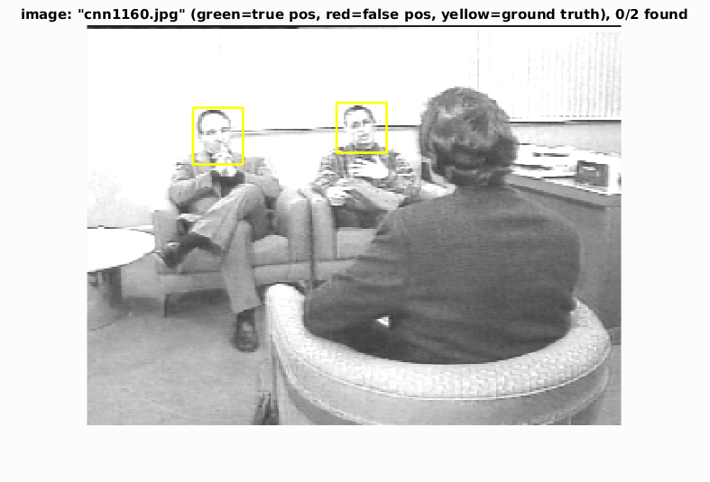
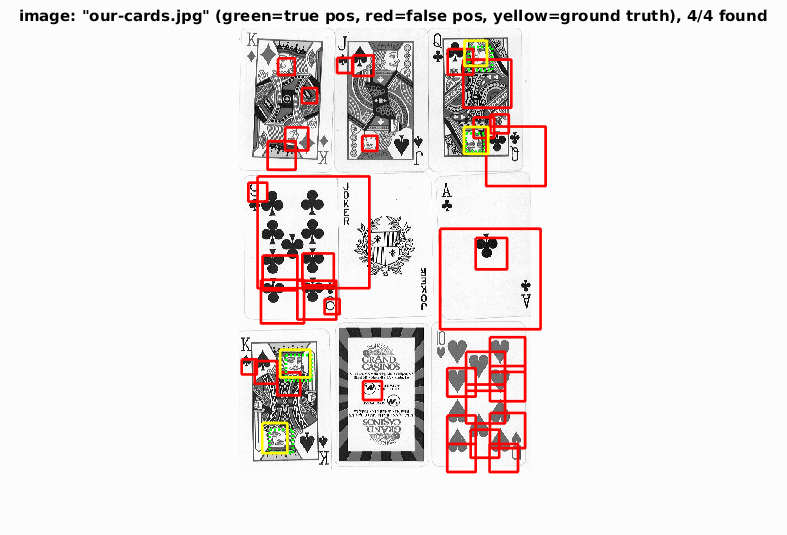
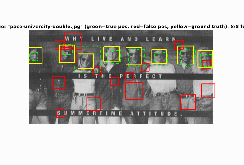
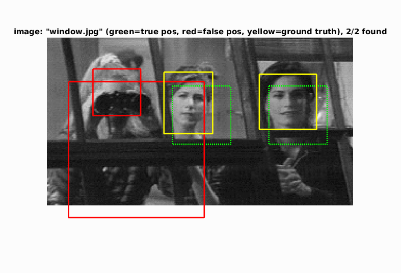
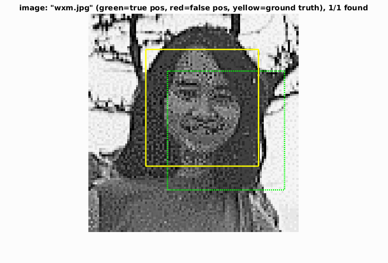
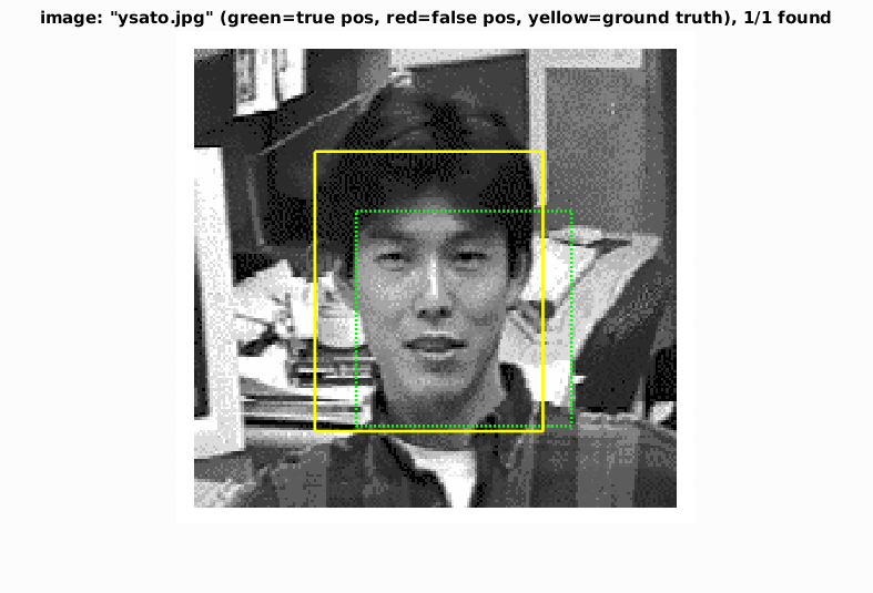
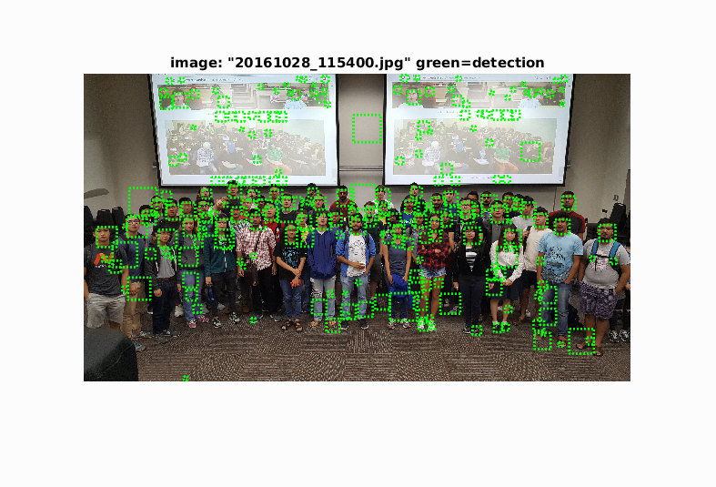
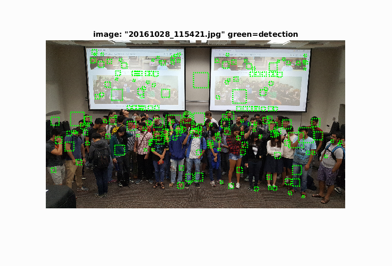
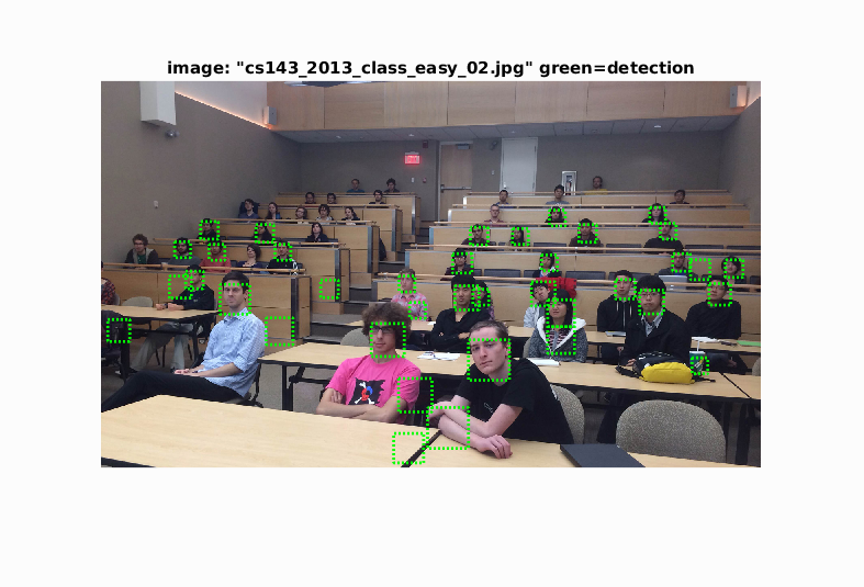
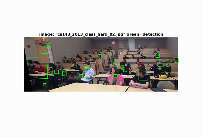
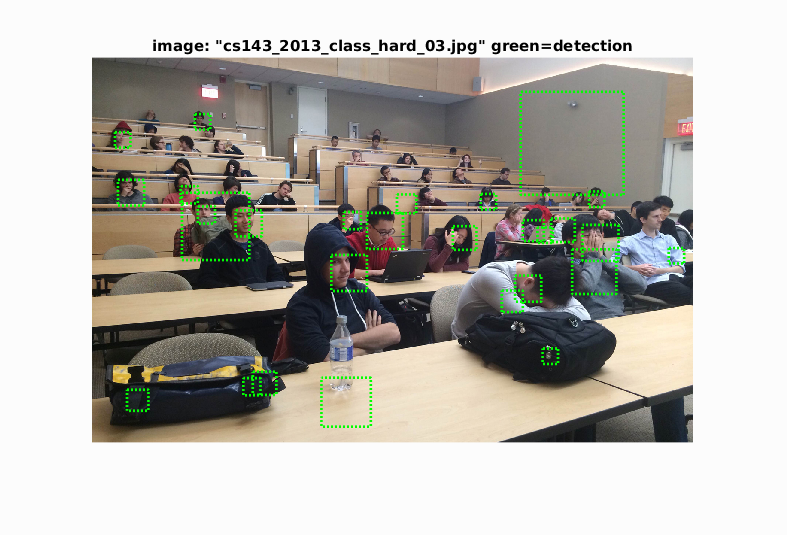
Classroom images
These are the detections on the extra test images using a higher confidence threshold (0.8).
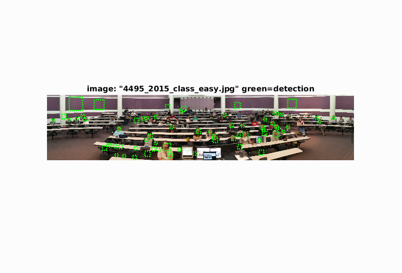
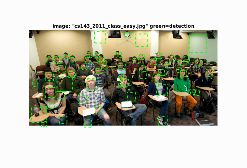
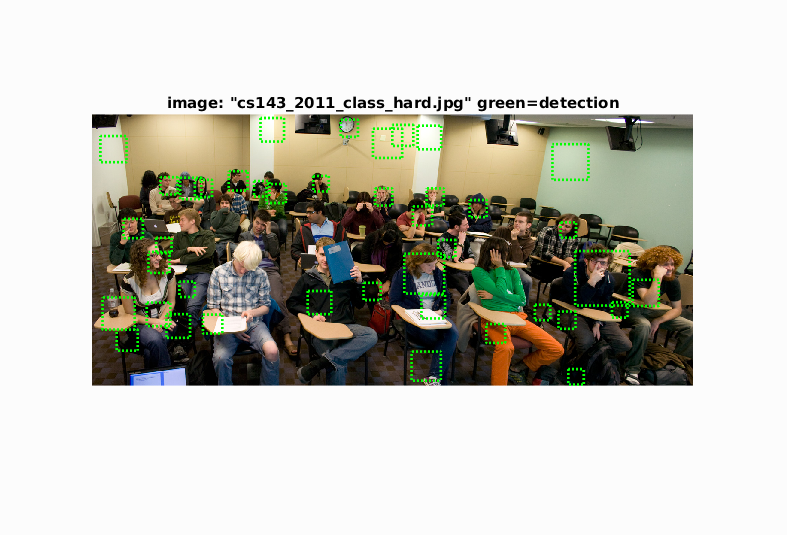
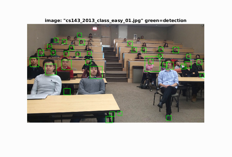

|