Face Detection Project

Project 5 / Face Detection with a Sliding Window

In this project I will train a SVM to detect faces using a sliding window of HoG features.

Pipeline

The pipeline of this project has four major steps described below.

Note that I didn't change starting parameters, that is I use the HoG cell size 6 and a template size of 36x36 pixels.

Getting Positive Features

The first step involve creating positive examples by extracting the HoG features from faces.


  hog = vl_hog(image, feature_params.hog_cell_size);

Here and for the rest of the code I will use the default Vlfeat HoG algorithm "UoCTTI".

Getting Negative Features

Next step is to extract the negative examples, i.e. none-faces. This is done by randomly selecting around 15000 patches from 274 scenes not containing faces. These patches are then turned into HoG features. Since all training faces are in grayscale we will convert all patches to grayscale first.


  hog = vl_hog(image, feature_params.hog_cell_size);
   [row_max, col_max, f_size] = size(hog);


   X = 1:feature_params.hog_cell_size:row_max - feature_params.hog_cell_size - 1;
   Y = 1:feature_params.hog_cell_size:col_max - feature_params.hog_cell_size - 1;
   num_x = min(N,size(X,2));
   num_y = min(N,size(Y,2));
   for x=X(randperm(size(X,2), num_x))
       for y=Y(randperm(size(Y,2), num_y))
           patch = hog(x:x+feature_params.hog_cell_size - 1, y:y+feature_params.hog_cell_size - 1, :);
           features_neg = [features_neg; patch(:)'];
       end
   end

The code above samples up to N^2 random non-overlapping patches from each images. With N=9 I could extract around 15000 examples.

Training SVM

Thanks to Vlfeat training an SVM is very straight forward. I concatenate the two sets of postive and negative examples and assign positive the label 1 and the negative the label -1.


  lambda = 0.00001;
  features = [features_pos' features_neg'];
  labels = [ones([size(features_pos, 1) 1]); -1 *ones([size(features_neg, 1) 1])];
  [w b] = vl_svmtrain(features, labels, lambda);

I used lambda = 0.00001 to get the best performance.

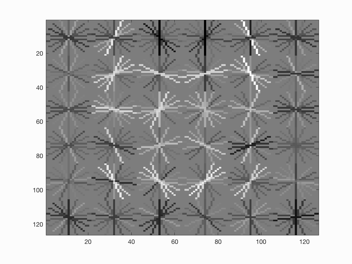
The image shows the learned HoG template.

Detector

The last step of the pipeline is to use a sliding window and our trained SVM to detect faces in test images. My detector runs an overlapping sliding window over around 10 different scales on the image.

  
    % create hog and create a sliding window
    hog = vl_hog(scaled_img, feature_params.hog_cell_size);
    for y=1:STEP_SIZE:size(hog,1) - feature_params.hog_cell_size - 1
        for x=1:STEP_SIZE:size(hog, 2) - feature_params.hog_cell_size - 1

            patch = hog(y:y+feature_params.hog_cell_size - 1, x:x+feature_params.hog_cell_size - 1,:);
            patch = patch(:)';
            class = w' * patch' + b';

            % if certainty is bigger than threshold save boundry.
            if class > THESHOLD_CONF
                cur_bboxes = [cur_bboxes; floor(feature_params.hog_cell_size * SCALE *
                  [x y (x + feature_params.hog_cell_size - 1) (y + feature_params.hog_cell_size - 1)])];
                cur_confidences = [cur_confidences; class];
                cur_image_ids = [cur_image_ids; test_scenes(i).name];
            end

        end
    end

If for a tested patch the SVM returns a value larger than THESHOLD_CONF it is considered a postive match. I used THESHOLD_CONF = 0.2 to get the best results. After detecting all bounding boxes for different scales I run the given non-maximum suppression to get only the best detections. If I wished to decrease the false positives it is just at matter of increasing THESHOLD_CONF.

Results

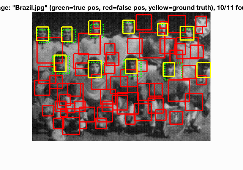
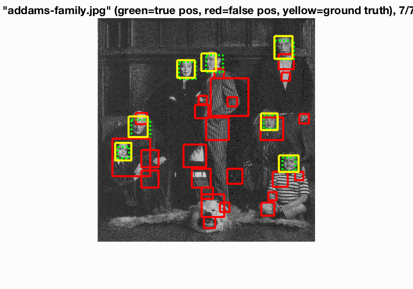
The average precision of my pipeline was 79.6%. Below are some examples and the precision-recall chart.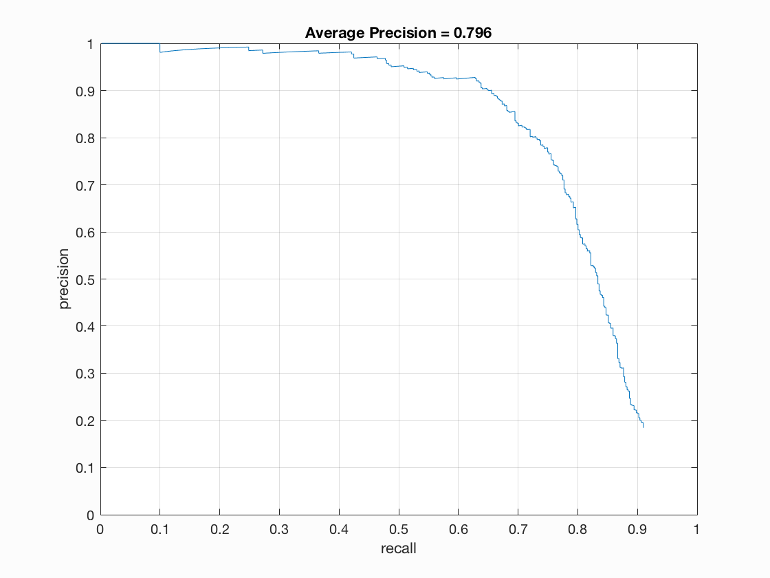

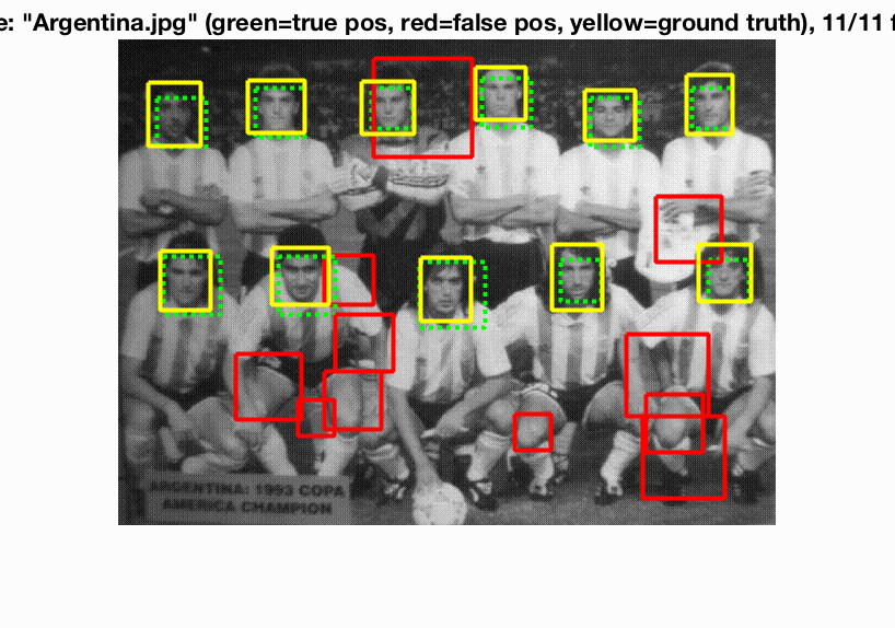
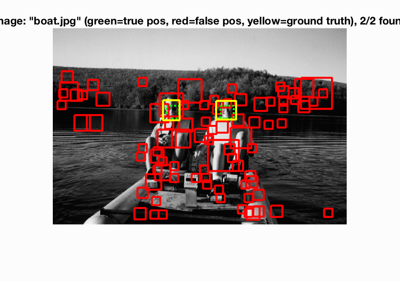
Below is a collection of example results. Notice that by increasing the THESHOLD_CONF we will reduce the number of false positives though this will decrease the average precision as well. As seen in the examples below my pipeline yields quite the number of false positives. I understand the wording in the problem description that this was fine and preferred over a configuration with less average precision but with less false positives.

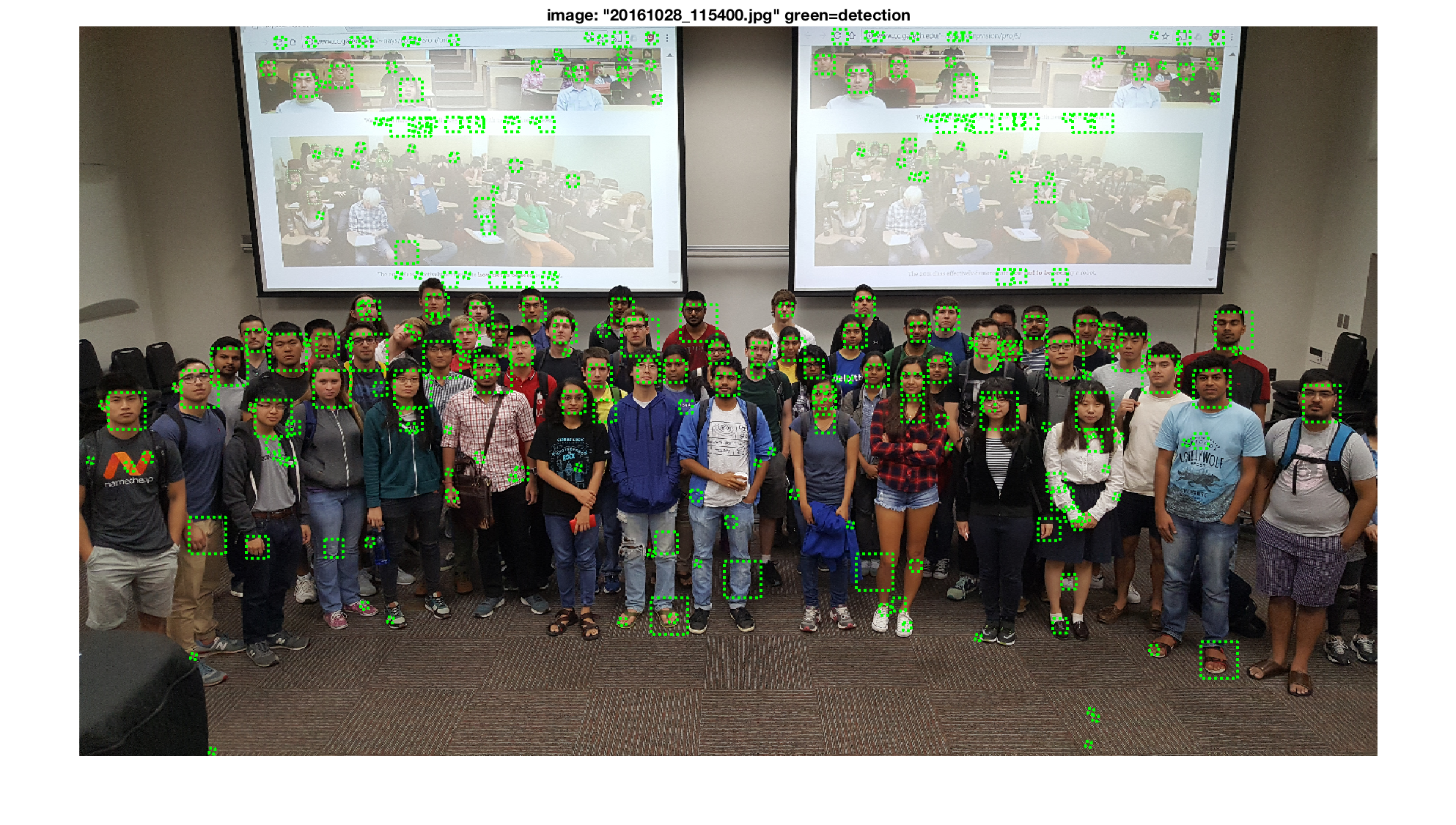
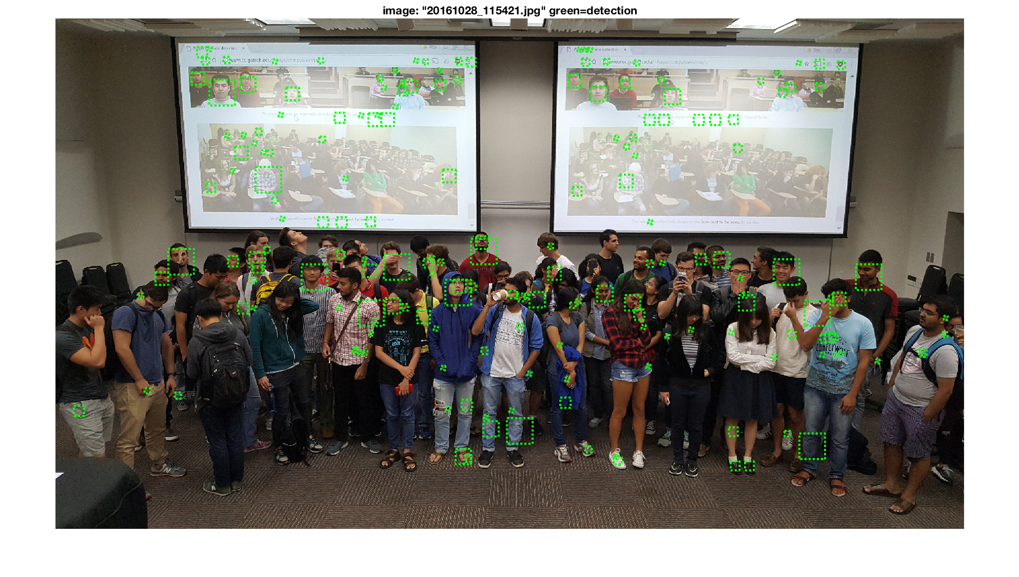
Example results

The top four images uses the threshold 0.2 while the two lower uses the threshold 0.7.

Erik Gartner