Project 5: Face detection with a sliding window
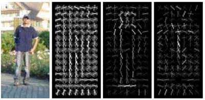
Figure-1: Histogram of Gradients (HoG) representation.
In this project, we implement the simpler (but still very effective!) sliding window detector of Dalal and Triggs 2005. Dalal-Triggs focuses on representation more than learning and introduces the SIFT-like Histogram of Gradients (HoG) representation (as in the Figure-1). We implement the detection pipeline, though -- handling heterogeneous training and testing data, training a linear classifier (a HoG template), and using our classifier to classify millions of sliding windows at multiple scales. Fortunately, linear classifiers are compact, fast to train, and fast to execute. A linear SVM can also be trained on large amounts of data, including mined hard negatives. Here is the outline of this project;
- Part I: Positive Features
- Part II: Random Negative Features
- Part III: Classifier Training
- Part IV: Run Detector
- Part V: Graduate and Extra Credit Works
Part I: Positive Features
Load cropped positive trained examples (faces) and convert them to HoG features with a call to vl_hog. We are provided with a positive training database of 6,713 cropped 36x36 faces from the Caltech Web Faces project. We arrived at this subset by filtering away faces which were not high enough resolution, upright, or front facing. get_positive_features.m file is implemented for this part as presented in the following code block.
function features_pos = get_positive_features(train_path_pos, feature_params)
image_files = dir( fullfile( train_path_pos, '*.jpg') ); %Caltech Faces stored as .jpg
N = length(image_files);
D = (feature_params.template_size / feature_params.hog_cell_size)^2 * 31;
features_pos=zeros(N,D);
for i=1:N
    I=single(imread(['../data/caltech_faces/Caltech_CropFaces/' image_files(i).name]))/255;
    HOG=vl_hog(I, feature_params.hog_cell_size);
    features_pos(i,:)=reshape(HOG,1,D);
end
Part II: Random Negative Features
In this section, we extract negative samples that do not contain faces. To extract enough samples from limited number of negative images, we extract 36x36 image patches randomly from each scaled version of images. For the initial step, we extract 10960 negative samples including 8 samples for each scale and 5 scales varying between 1 - 0.6561 for each image. If from a scaled version of image does not include enough samples, the remaining patches are extracted from other images. get_random_negative_features.m file is implemented for this part as presented in the following code block.
function features_neg = get_random_negative_features(non_face_scn_path, feature_params, num_samples)
image_files = dir( fullfile( non_face_scn_path, '*.jpg' ));
N = length(image_files);
D = (feature_params.template_size / feature_params.hog_cell_size)^2 * 31;

num_scales=5;
img_per_scale=ceil(num_samples/N/num_scales);
num_sample_truncate=0;% sample count that cannot be extracted from previous image. So extract from next image.
scale_factor=.9;
num_features = 0;
features_neg=zeros(img_per_scale*N*num_scales,D);
for i=1:N
    I=single(imread([non_face_scn_path '/' image_files(i).name]))/255;
    if(size(I,3) > 1)
        I = rgb2gray(I);
    end
    sI = I;

    nS=0;
    while nS < num_scales
        HOG = vl_hog(single(sI),feature_params.hog_cell_size);
        hog_size = size(HOG);

        if(hog_size(1)<=6 || hog_size(2)<=6)
            num_sample_truncate=num_sample_truncate+(num_scales-nS)*img_per_scale;
            break;
        end

        indices=1:( (hog_size(1)-5) * (hog_size(2)-5) );
        indices=indices(randperm(length(indices)));
        num_sample_truncate=num_sample_truncate+img_per_scale;

        scale_sample=num_sample_truncate;
        if numel(indices) < num_sample_truncate
            scale_sample=numel(indices);
        end

        for j=1:scale_sample
             num_features = num_features +1;
             index=indices(1);
             rX = ceil(index/(hog_size(2)-5));
             rY = mod(index-1,hog_size(2)-5)+1;
             hog_sample = HOG(rX:rX+5,rY:rY+5,:);
             hog_vector = hog_sample(:);
             features_neg(num_features,:) = hog_vector;
             num_sample_truncate=num_sample_truncate-1;
             indices(1)=[];
        end

        sI = imresize(sI,scale_factor^(num_scales-nS));
        nS=nS+1;
    end
end
Part III: Classifier Training
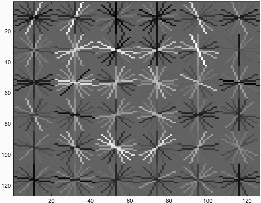
Figure-2: Trained HoG template.
This part is the most straight forward section. We used built-in training method 'vl_svmtrain' function in vlfeat library. We train a linear classifier from the positive and negative examples with a call to vl_trainsvm as in the following code stub.
function [w,b]=classifier_training(features_pos,features_neg,lambda)
X=[features_pos;features_neg];
Y=[ones(size(features_pos,1),1);-1*ones(size(features_neg,1),1)];
[w,b]=vl_svmtrain(X', Y, lambda);
end
After training we get HoG template presented in Figure-2. It seems we get a successful training template. Our initial classifier performance on train data is as follows;
  accuracy:   0.998
  true  positive rate: 0.380
  false positive rate: 0.001
  true  negative rate: 0.619
  false negative rate: 0.000
Part IV: Run Detector
In this section, we present the detection of test set. For each image, we run the classifier at multiple scales varying from 1.2 to smallest patch size which is 36x36. After getting all detection results, we run the non_max_supr_bbox to remove duplicate detections. Figure-3 and Figure-4 present the precision by recall changes and correct detections (recall) by false positive changes, respectively. We get following precision recall curve by using a lambda of 0.0001 and a threshold of 0.8 for linear svm score. It is worth to note that we use 6 pixel cell size and detector step for this result. As stated above, we use 10,960 negative samples and 6,713 positive samples for training. The average precision is 86.1% for these settings. We give the implementation of this section in following code block.
function [bboxes, confidences, image_ids] = run_detector(test_scn_path, w, b, feature_params)
    image_files = dir( fullfile( test_scn_path, '*.jpg' ));
    N=length(image_files);
    bboxes = zeros(0,4);
    confidences = zeros(0,1);
    image_ids = cell(0,1);
    scale_factor=.9;
    for i = 1:N
        I_org=single(imread([test_scn_path '/' image_files(i).name]))/255;
        name=image_files(i).name;
        cur_detections = 0;
        cur_confidences = zeros(0,1);
        cur_bboxes = zeros(0,4);
        cur_image_ids = cell(0,1);

        scale=1.2;
        I = imresize(I_org,scale);
        while (size(I) > feature_params.template_size) == [1 1]
            [scaled_detections, scaled_bboxes, scaled_confidences, scaled_image_ids] = run4scale(I, name, feature_params,w,b);
            cur_confidences = [cur_confidences; scaled_confidences];
            cur_bboxes = [cur_bboxes; (scaled_bboxes./scale)];
            cur_image_ids = [cur_image_ids; scaled_image_ids];
            cur_detections = cur_detections + scaled_detections;

            I = imresize(I,scale_factor);
            scale=scale*scale_factor;
        end

       [is_maximum] = non_max_supr_bbox(cur_bboxes, cur_confidences, size(I_org));

        cur_confidences = cur_confidences(is_maximum,:);
        cur_bboxes      = cur_bboxes(     is_maximum,:);
        cur_image_ids   = cur_image_ids(  is_maximum,:);


        bboxes      = [bboxes;      cur_bboxes];
        confidences = [confidences; cur_confidences];
        image_ids   = [image_ids;   cur_image_ids];

    end
end

function [scaled_detections, scaled_bboxes, scaled_confidences, scaled_image_ids] = run4scale(image, img_name, feature_params,w,b)
    THR=0.8;
    template_size=feature_params.template_size;
    hog_cell_size=feature_params.hog_cell_size;
    cell_step=6;
    D=(template_size / hog_cell_size)^2 * 31;

    HOG = vl_hog(image, hog_cell_size);
    hog_size = size(HOG) - cell_step;
    hog_mat = zeros(hog_size(1)*hog_size(2),D);
    scaled_bboxes = zeros(0,4);
    row = 1;
    for j = 1:hog_size(1)
        for k = 1:hog_size(2)
            hog_mat(row,:) = reshape(HOG(j:(j+cell_step-1),k:(k+cell_step-1),:), [1 D]);
            window = hog_cell_size*[k j];
            scaled_bboxes(row,:) = [window (window+template_size-1)];
            row = row + 1;
        end
    end
    temp_confidences = hog_mat*w + b*ones([size(hog_mat,1) 1]);
    perm_conf_indices = temp_confidences >= THR;
    scaled_detections = sum(perm_conf_indices);
    scaled_bboxes = scaled_bboxes(perm_conf_indices,:);
    scaled_confidences = temp_confidences(perm_conf_indices,:);
    scaled_image_ids = repmat({img_name}, [scaled_detections 1]);
end

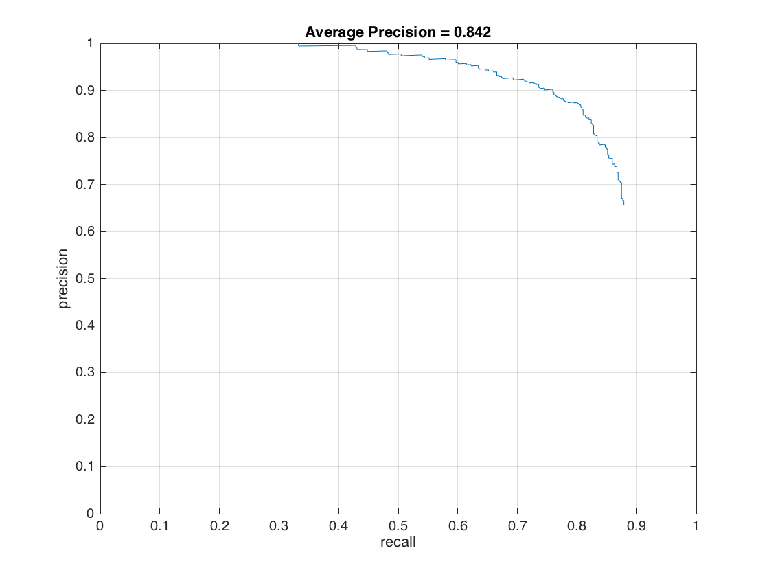
Figure-3: Precision recall |
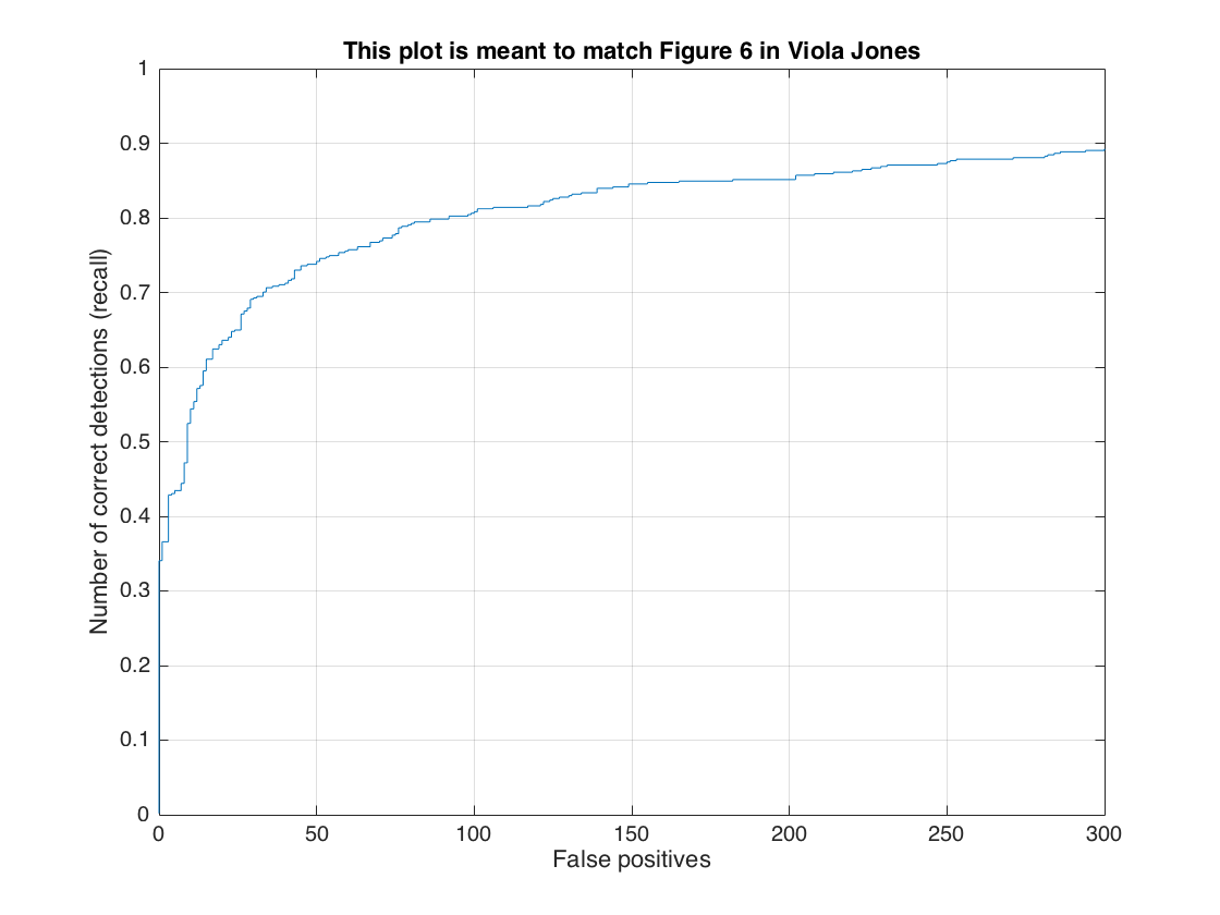
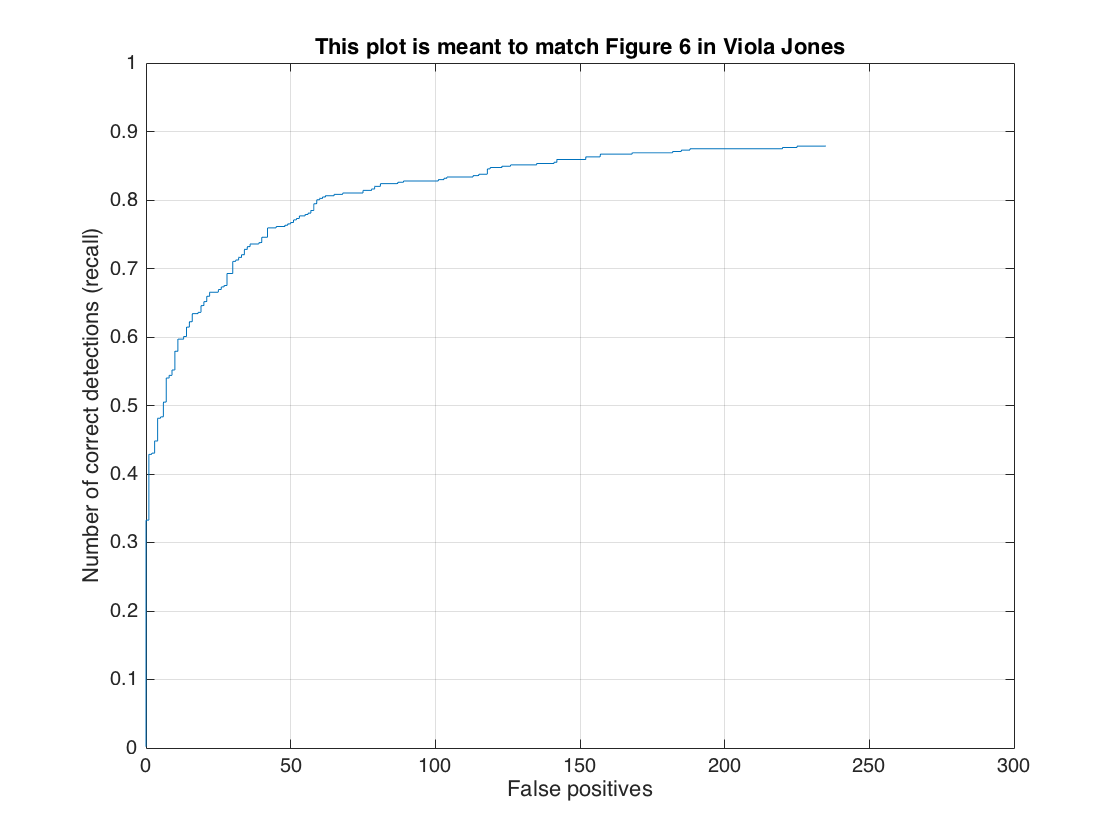
Figure-4: Recall by false-positives |
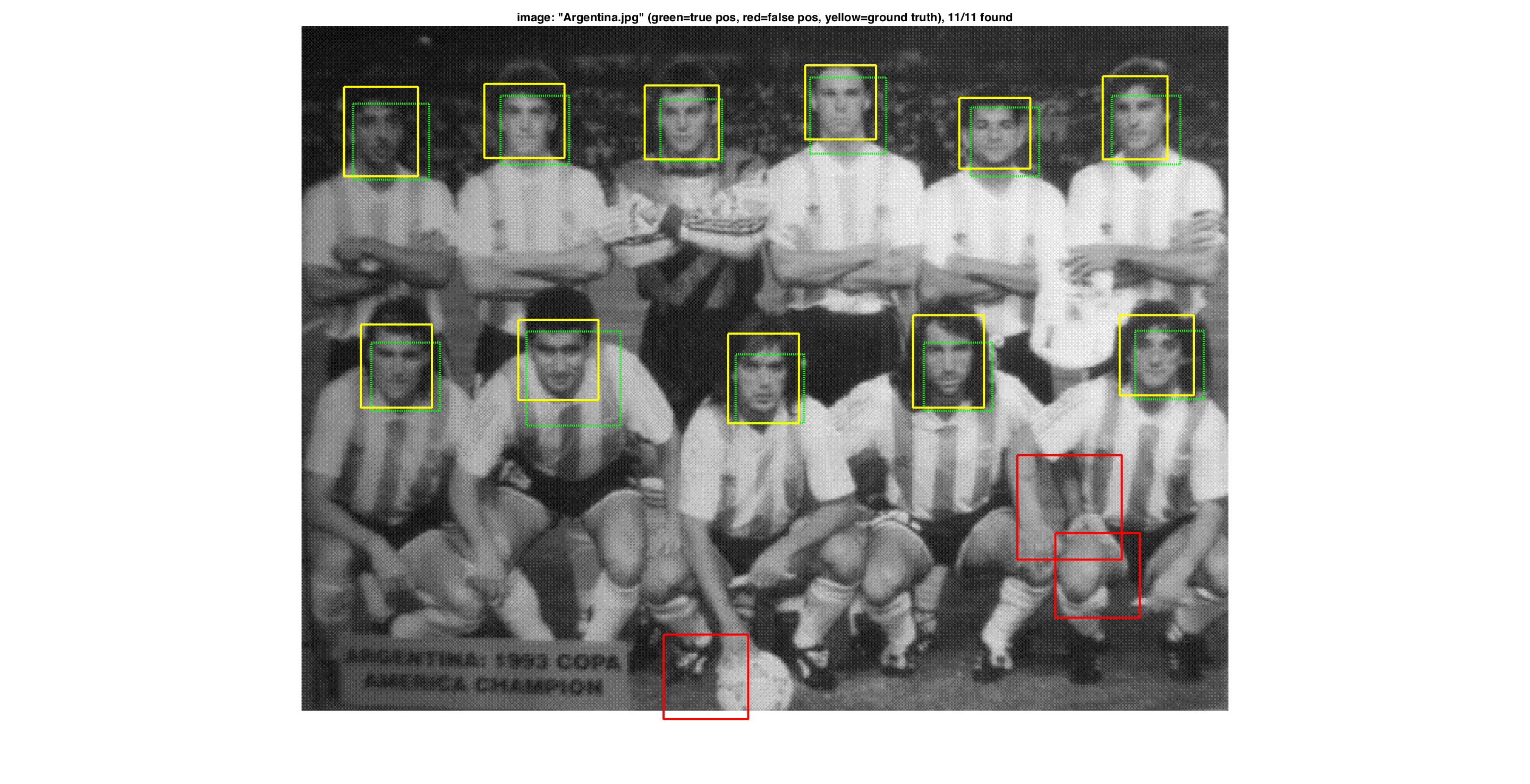
In the following figures we present a good example with no false-positives, a typical example with detected face and false-positives and finally a bad example with no detected face but many false-positives.
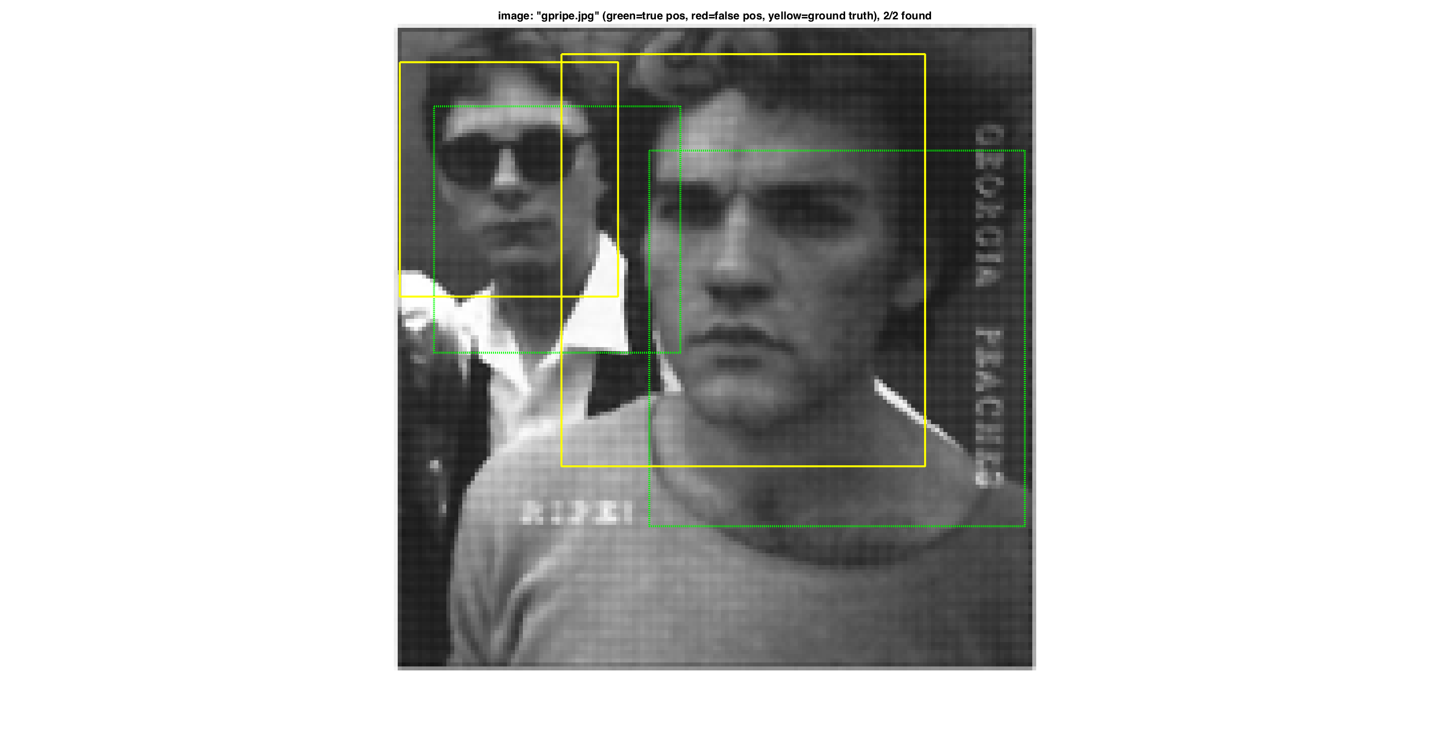
Figure-5: The good |
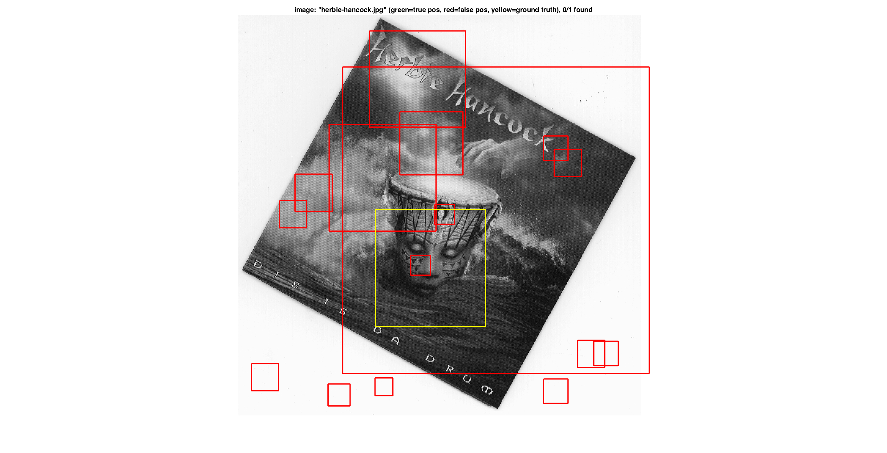
Figure-6: The bad. |
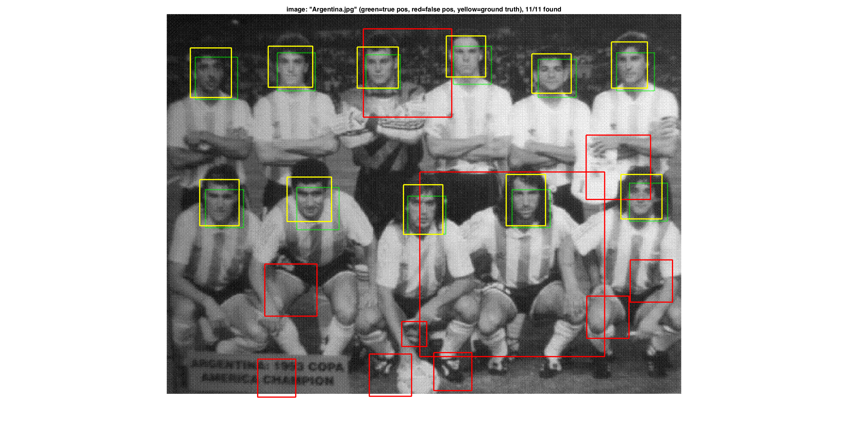
Figure-7: The typical. |
Part V: Graduate and Extra Credit Works
1- Find and utilize alternative positive training data: In this section, we present the detection results with the Labeled Faces in the Wild (LFW) dataset. To do this, we use the cropped version of the LFW dataset which includes only face part of each images in 64x64 size. This cropped version of LFW dataset can be found on Cropped LFW dataset To use this dataset in our experiments, we resize each face images to 36x36. We first train our model by using only LFW dataset, and then, we build a model by using Caltech Web Faces and LFW datasets together. Both HoG templates are presented in following Figure-8 and Figure-9, respectively.
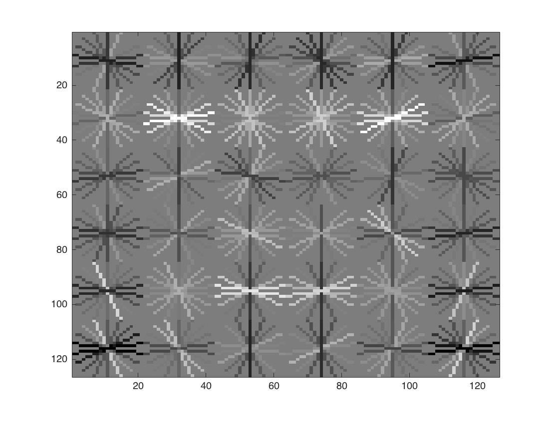
Figure-8: LFW HoG Template. |
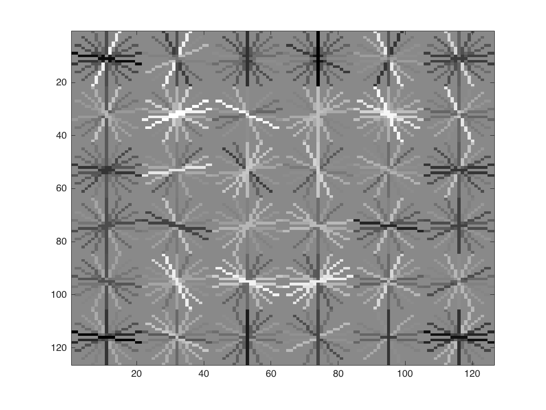
Figure-9: LFW and Caltech_CropFaces HoG Template. |
It is worth to note that we did not change any settings on classifier for initial tests. Hence, precision recall curve and recall false-positive results presented on Figure-10 and Figure-11 give us 57.7% of an average precision rate. We also present a good, bad and typical detection samples with these settings. Results have low average precision but also have low false positives.

Figure-10: Precision recall for LFW |
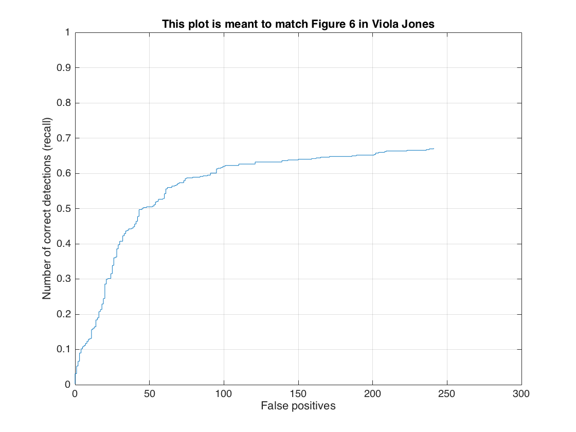
Figure-11: Recall by false-positives for LFW |
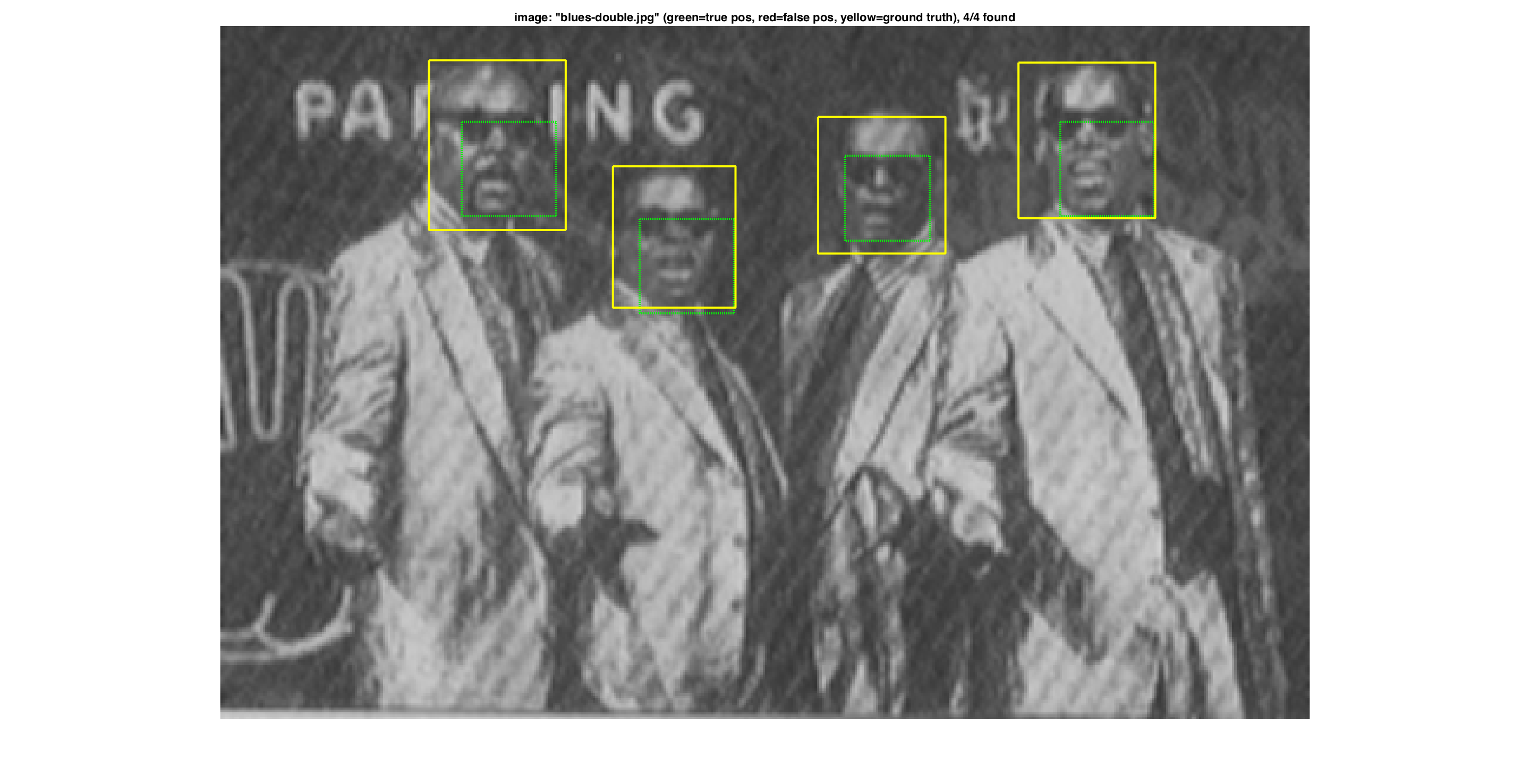
Figure-12: The good |
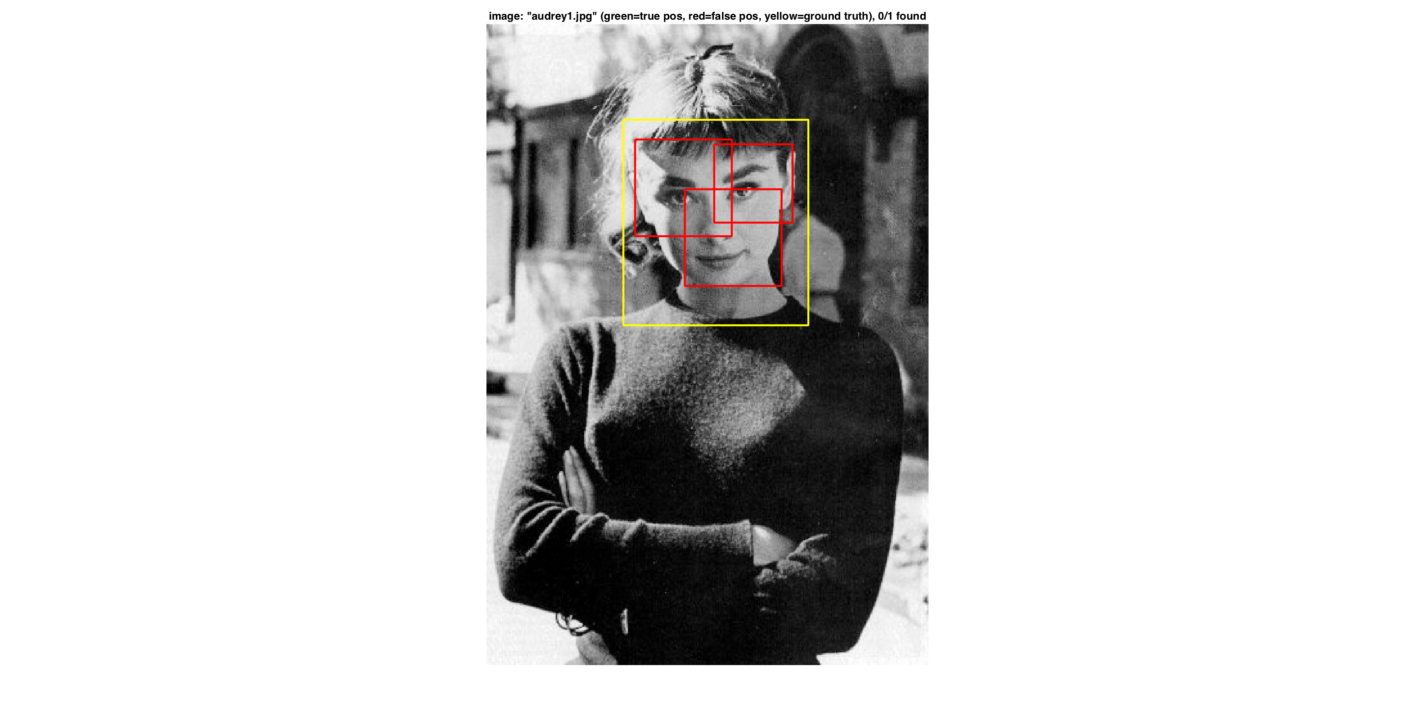
Figure-13: The bad. |
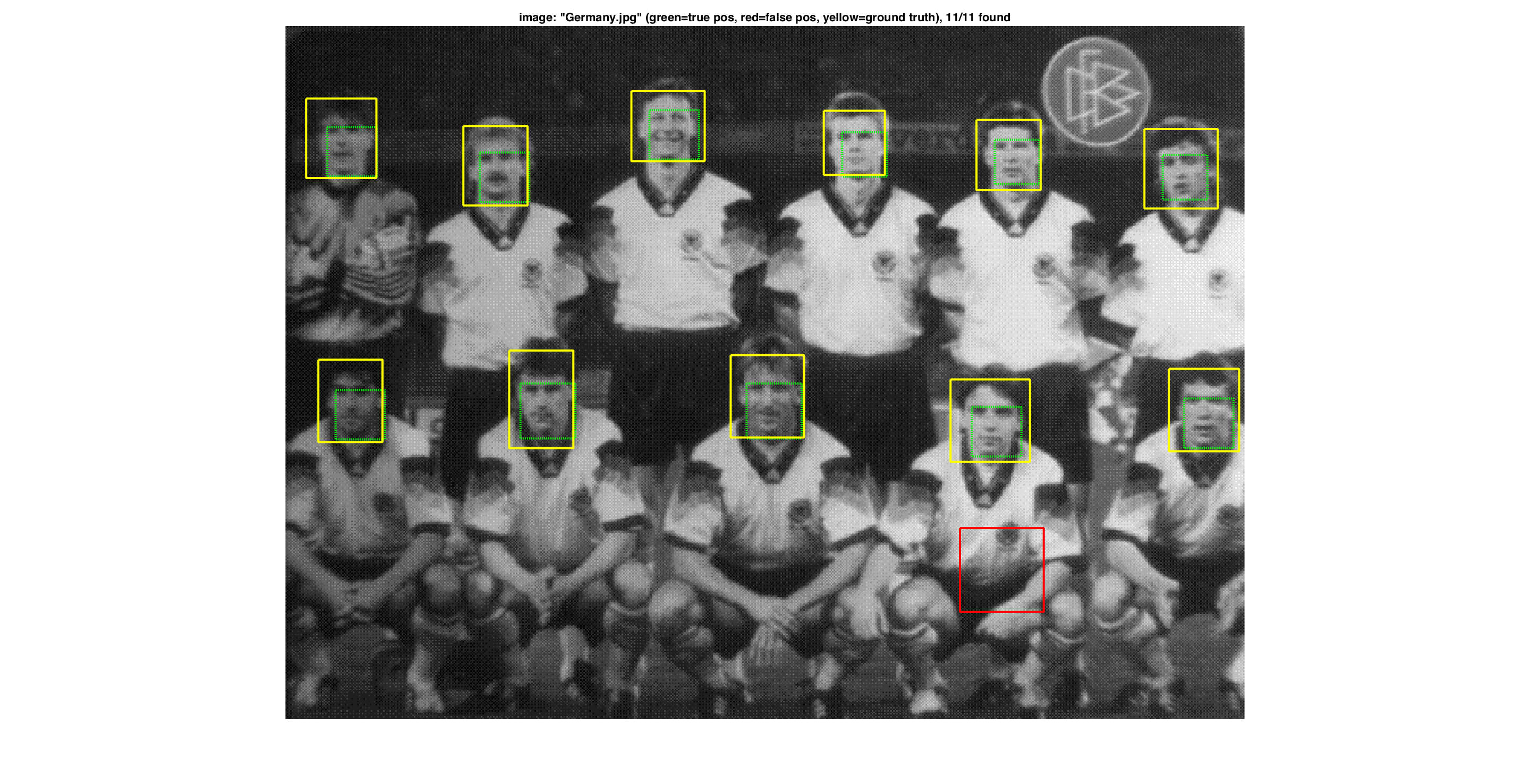
Figure-14: The typical. |
As an improvement, we decrease the threshold value used in svm detection from 0.8 to -0.3. Then, our average precision increase to 63.1%.
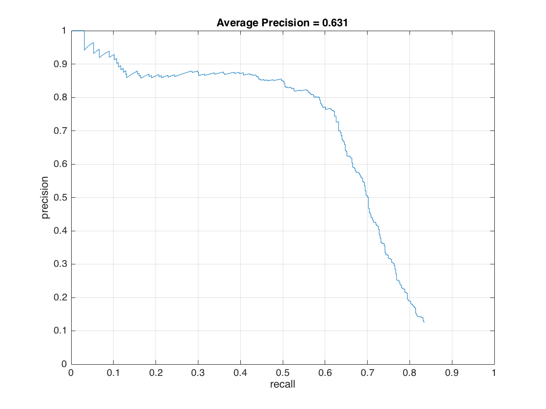
Figure-15: Precision recall for LFW. Theshold=-0.3 |
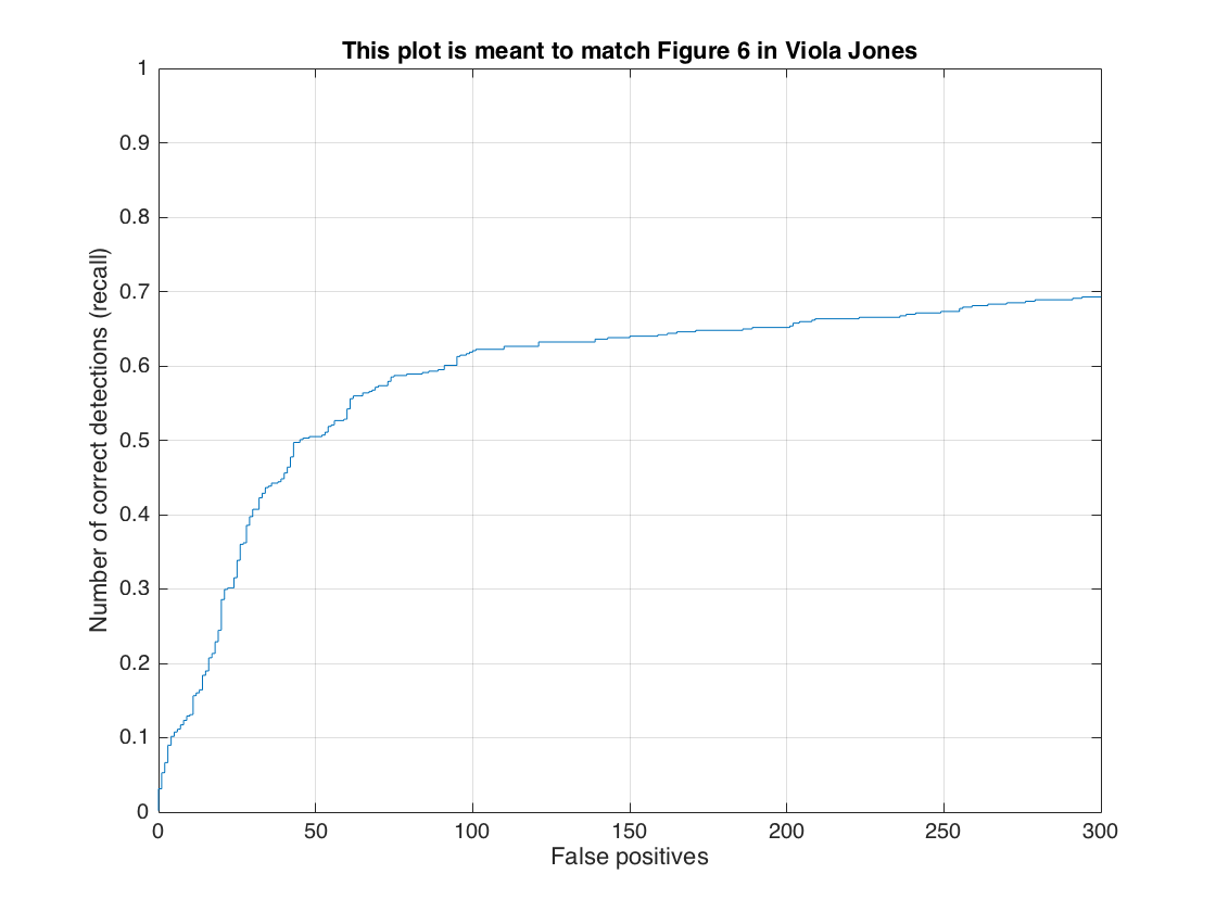
Figure-16: Recall by false-positives for LFW. Theshold=-0.3 |
As a final evaluation, we used HoG model built by both Caltech_CropFaces and LFW datasets. For this experiment, we keep the threshold value same as -0.3 and increase also the random negative samples from 10,960 to 20,000 since the positive samples are increased. Following figures show our results which have an average precision of 79.9%.
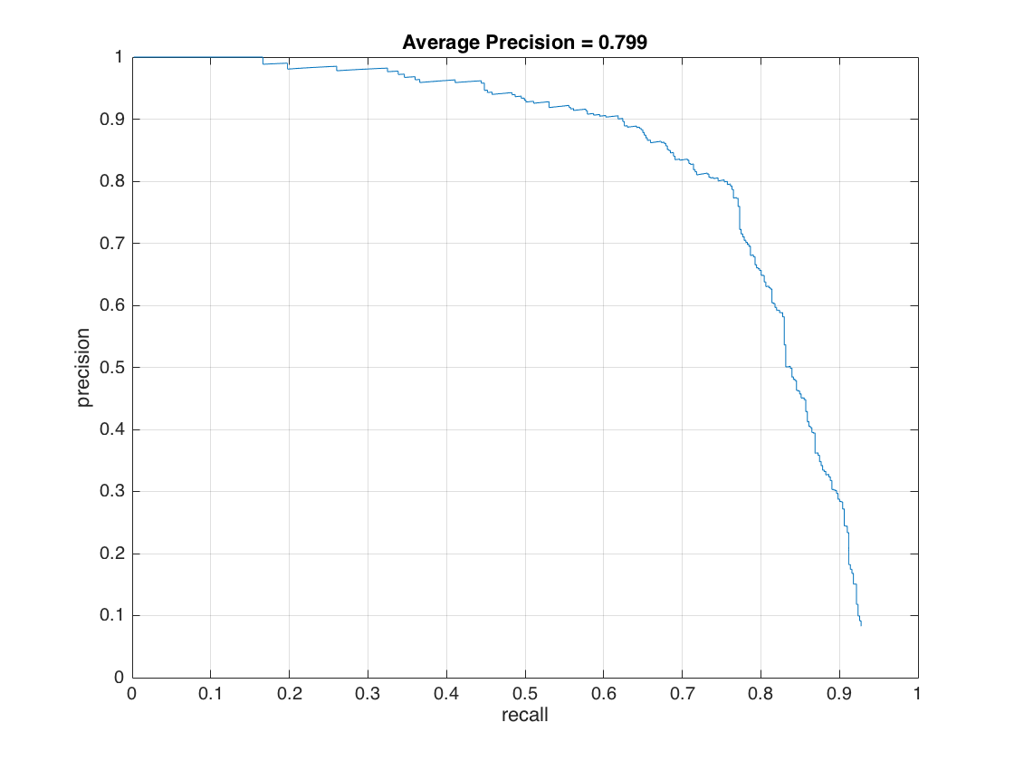
Figure-17: Precision recall for LFW and Caltech_CropFaces. Theshold=-0.3 |
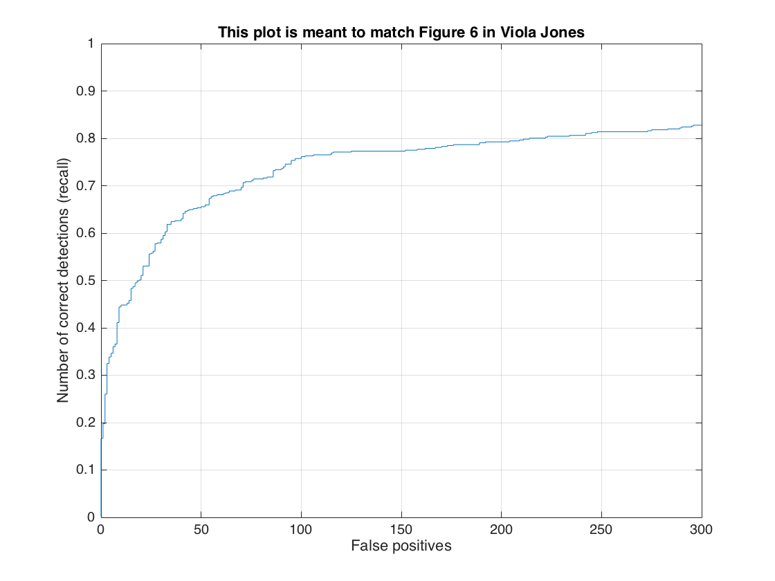
Figure-18: Recall by false-positives for LFW and Caltech_CropFaces. Theshold=-0.3 |
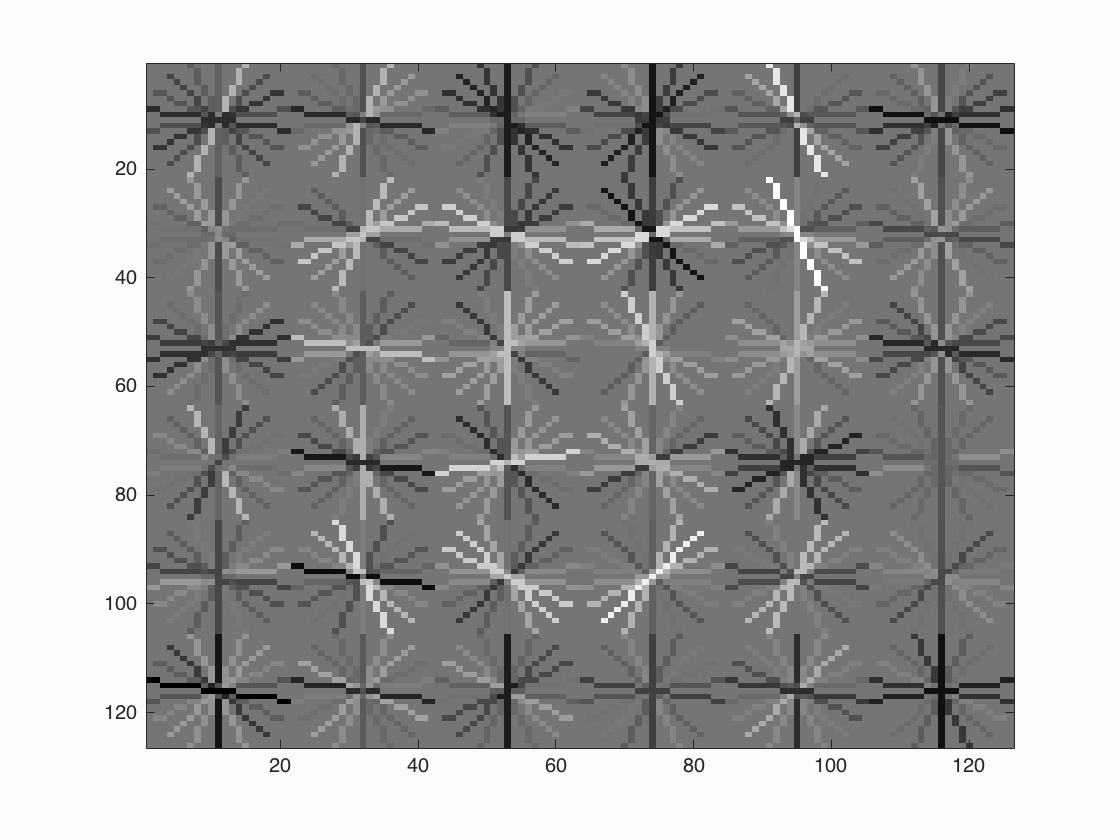
Figure-19: HoG template for 20000 negative samples and Caltech_CropFaces.
2- Utilize random negative samples: In this section, we present the detection results with the increased number of negative samples for only Caltech_CropFaces dataset. To do this, we only increase the number of random negative samples from 10,960 to 20,000. Figure-19 shows the trained HoG template for this setting. We got 84.2% average precision rate but with low false-positives. Following figures show precision recall curve and recall false-positive curve, and, also the typical result with lower false-positives.
|
|
3- Different feature set - Local Binary Patterns (LBP): In this section, we present the detection results with different set of features which previously used in face detection succesfully. For this purpose, we choose Local Binary Pattern (LBP) features, which is used in following paper for face detection and recognition purpose previously;
Ahonen, Timo, Abdenour Hadid, and Matti Pietikainen. "Face description with local binary patterns: Application to face recognition." IEEE transactions on pattern analysis and machine intelligence 28.12 (2006): 2037-2041.
Local Binary Pattern (LBP) features have performed very well in various applications, including texture classification and segmentation, image retrieval and surface inspection. The original LBP operator labels the pixels of an image by thresholding the 3-by-3 neighborhood of each pixel with the center pixel value and considering the result as a binary number. For this part of project, we employ similar approach by using built-in matlab function 'extractLBPFeatures()' with 18 pixels neighborhood and 3 pixels radius settings. We simply extract LBPs of given positive images and 36x36 random patches from negative examples and train a model. Our initial classifier performance on train data is as follows;
  accuracy:   0.964
  true  positive rate: 0.228
  false positive rate: 0.019
  true  negative rate: 0.735
  false negative rate: 0.018
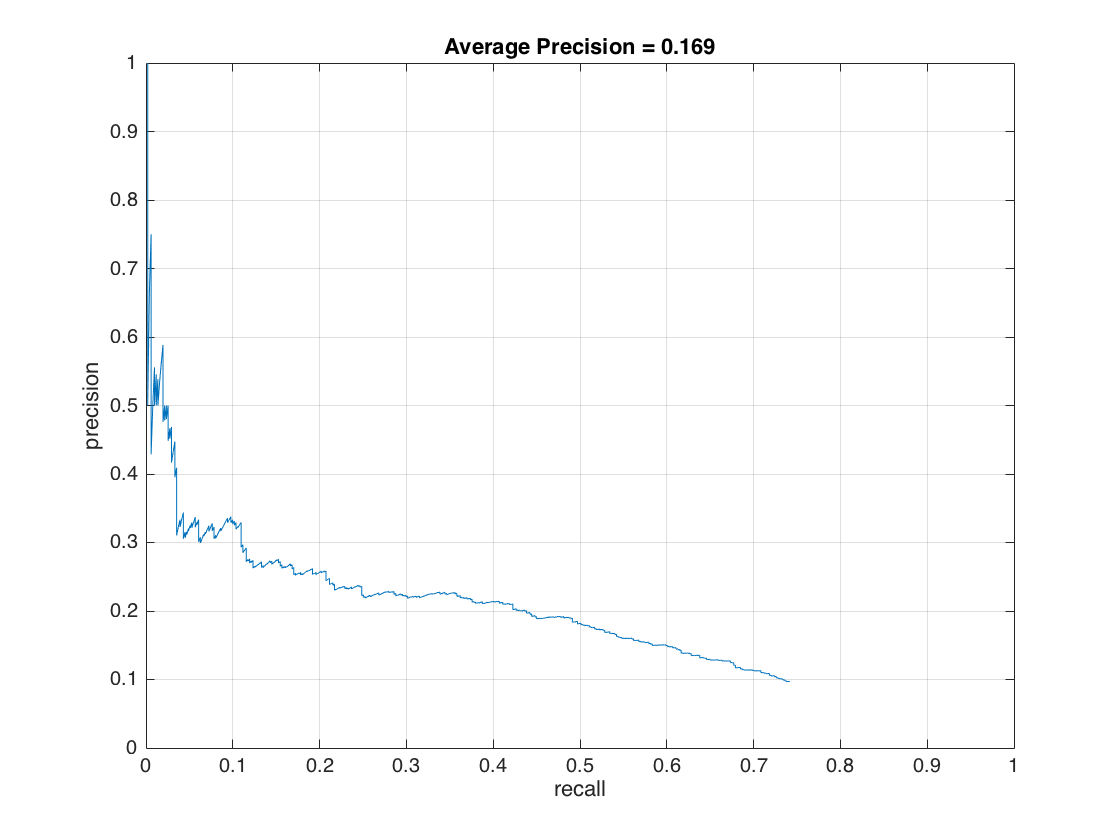
Figure-20: Recall by false-positives for Caltech_CropFaces with LBPs.
This initial performance result show that we have a reasonable face detection model. As a next step, we extract LBPs from 36x36 patches of given test images by sliding 18 pixels each time, and, compare the linear SVM score with the same threshold value we previously used (0.8). The modified version of the code for LBP is provided as a second code directory. The Figure-20 show that the LBPs have a 16.9% of an average precision on Caltech_CropFaces dataset with aforementioned settings. Test results do not give a high detection rate, but, LBP is presented as a successful face detection technique in above work.
It is worth to note that the running time of LBP features are very slow comparing with HoG features. Moreover, it is obvius that we can increase the accuracy by utilizing the free parameters also. However, because of the slowliness of the LBP features, different parameter utilization could not be performed at this time. On the other hand, the complex analysis, conducted on The Facial Recognition Technology (FERET) database, show that the LBP has successful results on given reference above.