Graham Wright

Single Scale Detection

As an intermediate step, I implemented a single scale face detection. In this version, we simply search for 36x36 faces in the test images using our HOG feature SVM. I achieved a maximum accuracy of 33.4%. I used this opportunity to find the top performing SVM lambda of 0.00001. We can expect a much higher accuracy when taking into account the different scalings of images; obviously faces are not only constrained to 36x36 pixel squares.

Multi Scale Detection

Our performance with a single scale was relatively poor, so we now implement multi scale detection to detect faces at multiple scales.

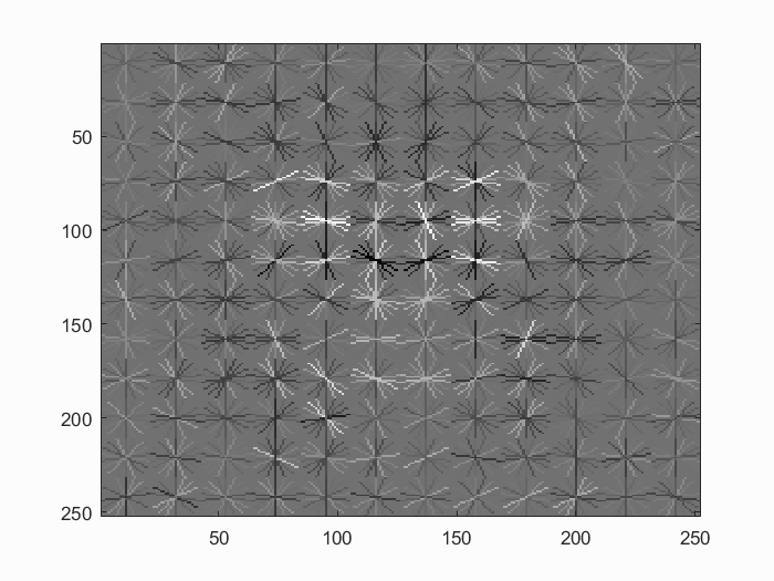
Hog features for a cell size of 3. We can start to see the face outline.

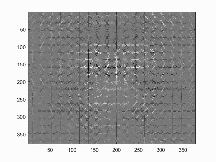
Hog features for a cell size of 2. Our smaller cell size allows us to create a finer face.

Parameter	Justification
Number of negative examples	I ended up using 10000 negative examples. Additional negative examples did not seem to have a noticeable impact on performance.
Negative examples scale sampling	When taking random samples from face-less images, I took them at multiple scales. The scales were recursively reduced by 60% for 5 iterations, starting at full scale. This hopefully gives a more representative view of non-face sliding windows.
Test image shifts	When evaluating the test image, the detection is limited to alignments of HOG cells. Although we are sampling at multiple scales, I added a single 18 pixel shift to augment the scaling in an attempt to cover more ground on the detection squares. It is run once with no shift and another time with the 18 pixel shift. This potentially had a very small boost in performance, moreso for runs with less scale iterations.
Test image scaling	When evaluating the test image, I took sliding windows at scale steps of 0.95, however I first started with scales of 1.2, 1.1, and 1. I recursively applied the scale step 77 times. Initially, a scale step of 0.9 was working well, but I ended up seeing a final boost of about 0.7% by adding in more scales.
Hog cell size	As is expected, decreasing from a HOG cell size from 6 to 4 to 3 improved results. The improvement from 6 to 4 was approximately 6%, while the improvement from 4 to 3 was approximately 1-2%. I did not see a significant improvement when dropping to a cell size of 2 when precision is already over 90%. A cell size of 2 also takes significantly longer than a cell size of 3. I could see some occasional improvements for lower accuracy bands (such as 80%).
SVM lambda	A value of 0.00001 turned out to be a very effective lambda for the SVM. This was a noticeable local maximum in my testing, giving a train accuracy of 1.
SVM detection prediction threshold	I mainly used a prediction threshold of -0.2. That is, I passed detections of > -0.2 to non maximum supression for the final face detection boundary boxes. A lower threshold ends up taking longer with little noticeable precision improvement, and a higher threshold tended to reduce precision.

This face detector took 34 minutes and 33 seconds to train and test. As a comparison, during testing, I could train an 82% detector in 4 minutes (0.7 scale step, 8 scale iterations, cell size of 6) and a 90.3% detector in 6 minutes and 9 seconds (0.7 scale step, 8 scale iterations, cells size of 4).

Examples

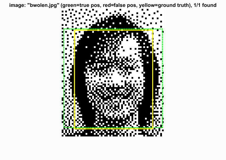
Blunders

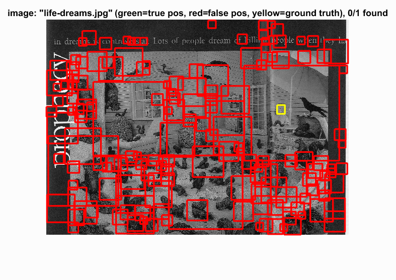
I don't even think I could get the one on the right correct myself...

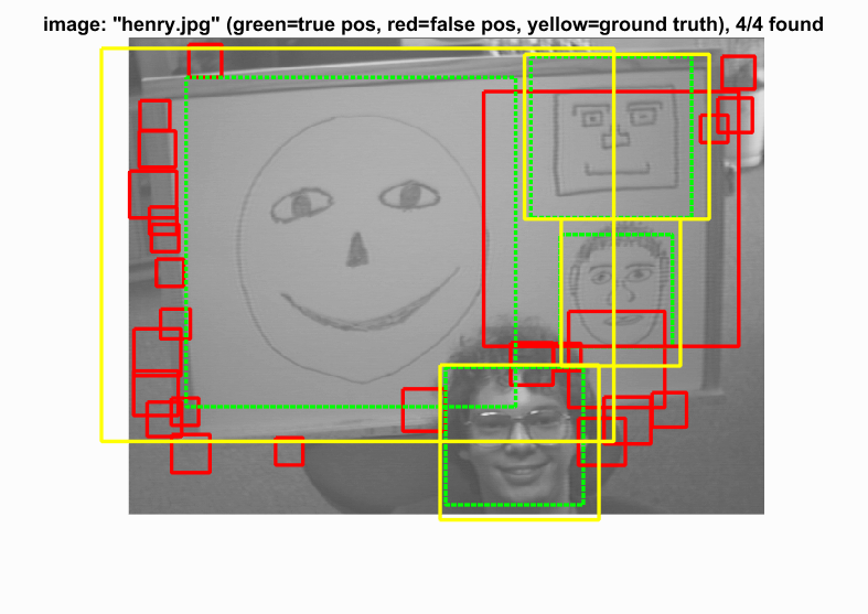
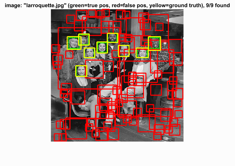
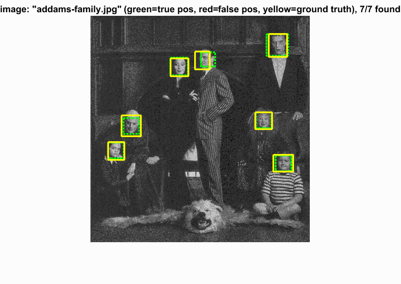
Success

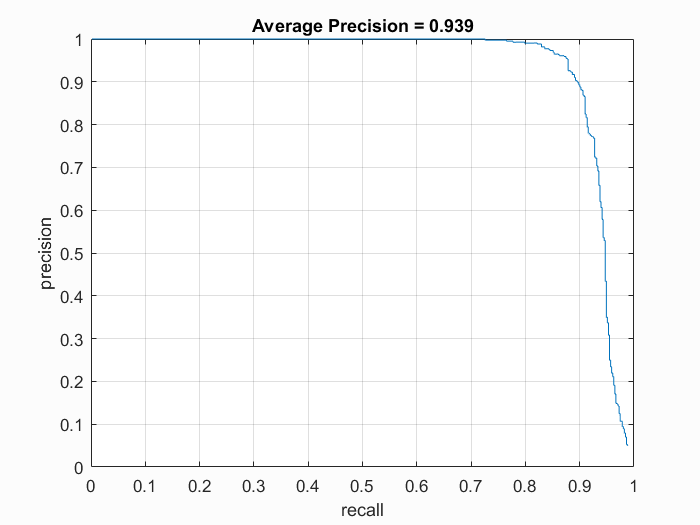
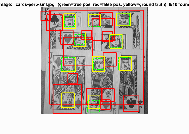
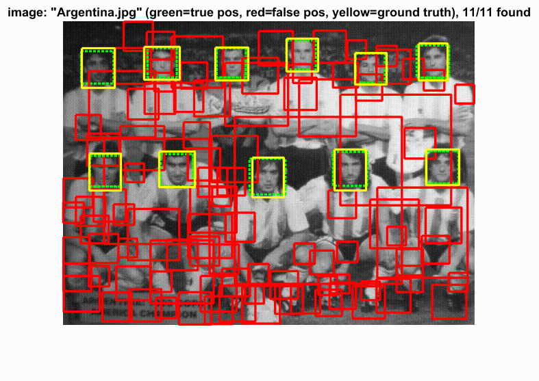
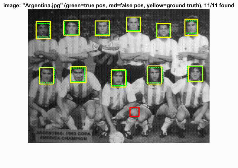
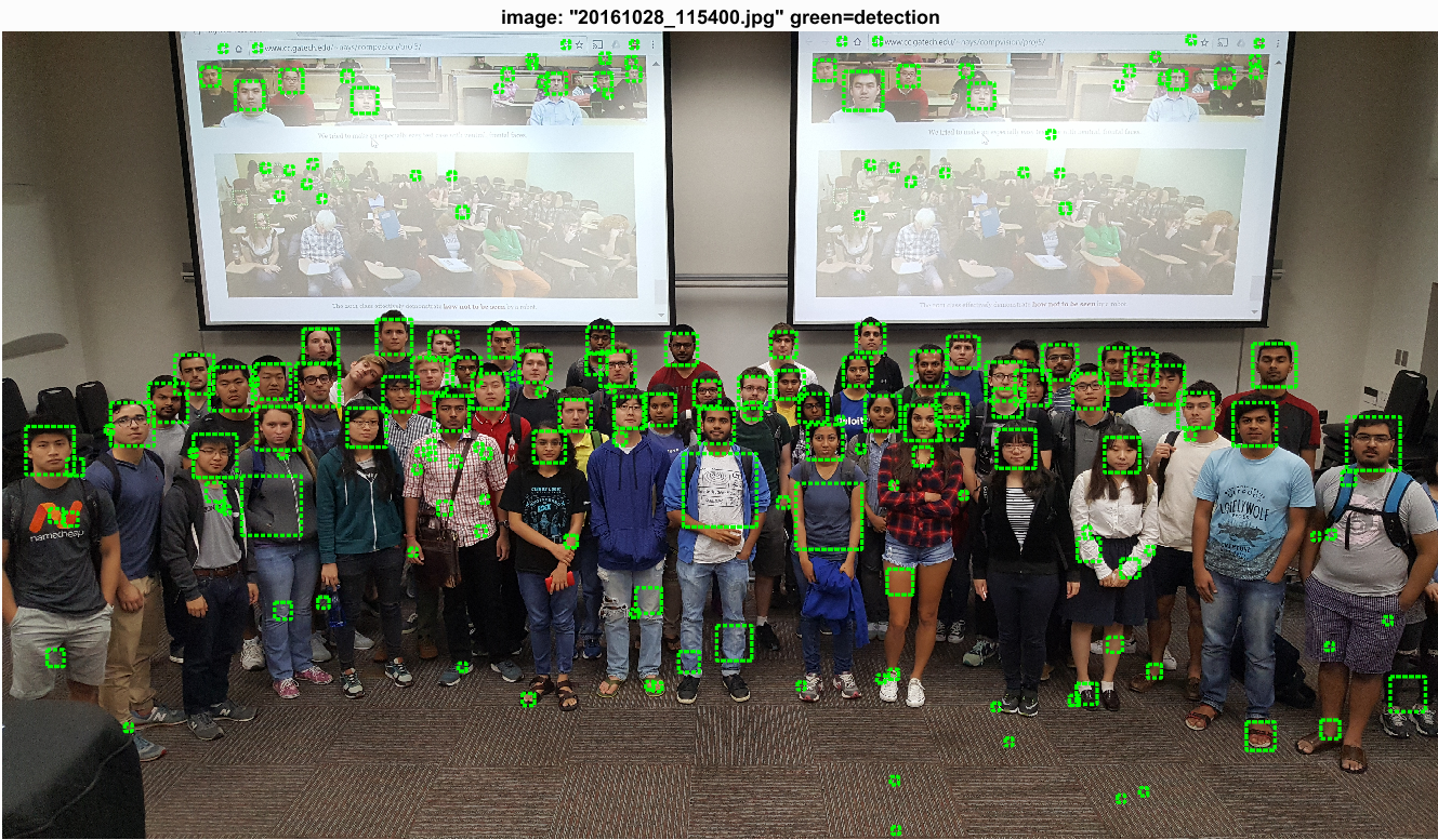
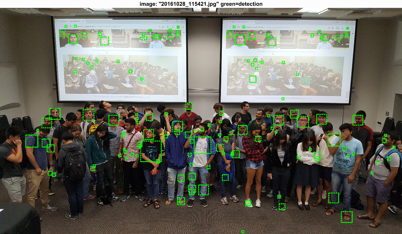
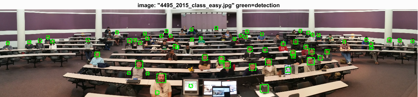
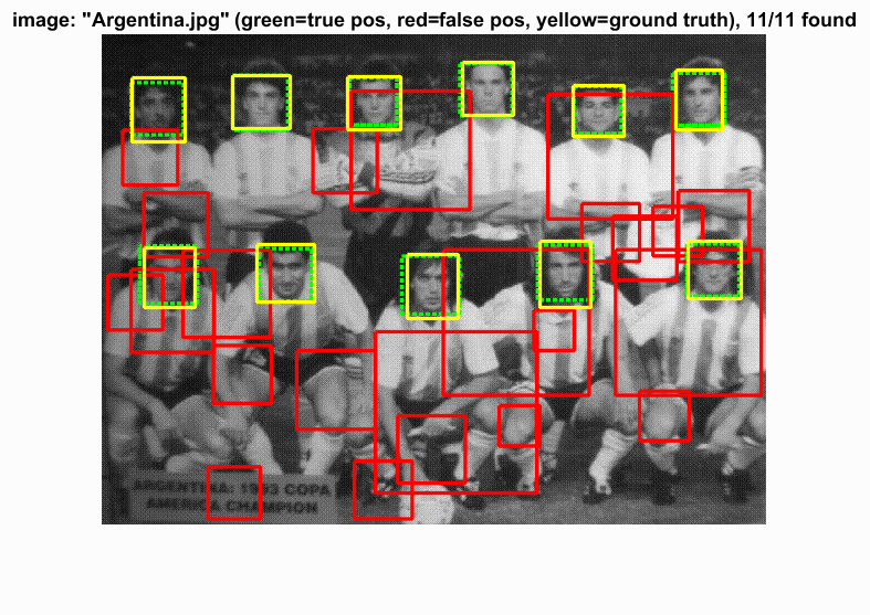
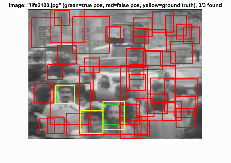
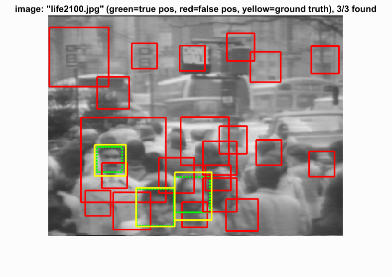
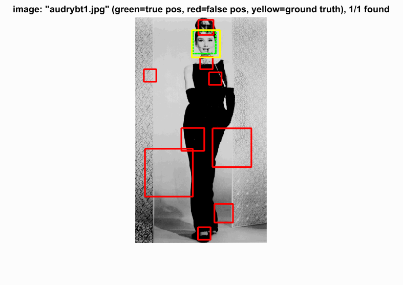
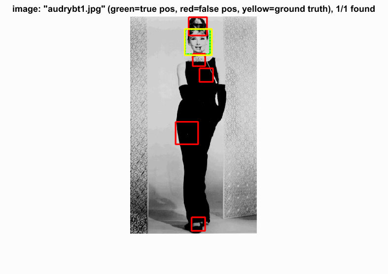
	As seen above, the detector that achieves an accuracy of 93.9% also produces a lot of false positives with a threshold of -0.2. On the left we have another image detected with a threshold of -0.2, and on the right we have an image detected with a threshold of 1.0. Thresholding at 1.0 hurts accuracy by about ~2-2.5% (here it is at 90.9%) but leaves us with much cleaner detections.

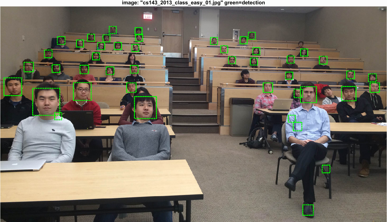
Extras

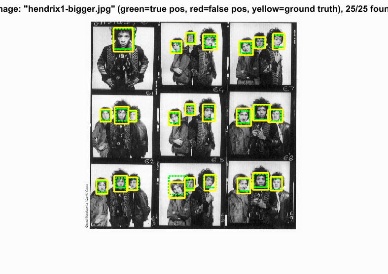
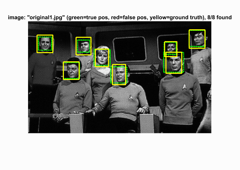
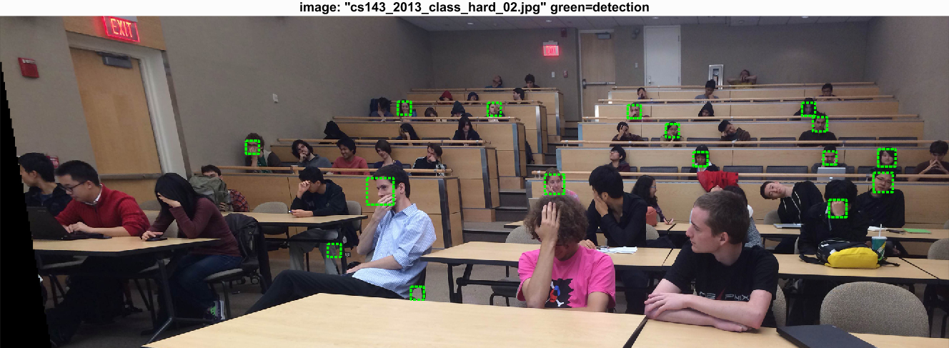
These images have been evaluated on the thresholded face detector to reduce false positives in the images.

There seems to be some difficulty with faces shown from the side. I think additional training data that emphasized different face perspectives could improve this performance. Clearly, this detector is very effective at faces which face forward.

Mining Hard Negatives

I also tested out some mining of hard negatives. After training the SVM, I again evaluated the SVM on random patches of negative images, this time at scale steps of 0.7 for 5 iterations. I configured the process to sample 5000 patches from each negative image and keep predictions that were greater than 0 (which there ended up being 1724 of). I used these positive prediction value patches as more negative training examples and retrained the SVM with these additional negatives. Overall, I did not see a noticeable impact on performance. I actually did manage to reach a higher average precision when testing this technique, however it is not clear if this technique was the reason I reached this precision as each run has inherent variability due to the randomness of the negative example gathering and SVM training. Nevetheless, this used the same configuration as the previous top performing result (of course other than the hard negative mining). Hard negative mining does not add too much computation time; in my experience it ranged from 1-2 additional minutes depending on the number of hard negatives mined.

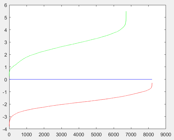
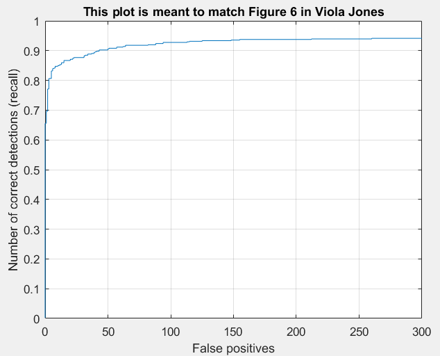
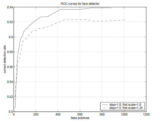
And here you will find the SVM boundary as well as the Viola Jones figure comparison. Notice that the SVM boundary is very divisive in this run.

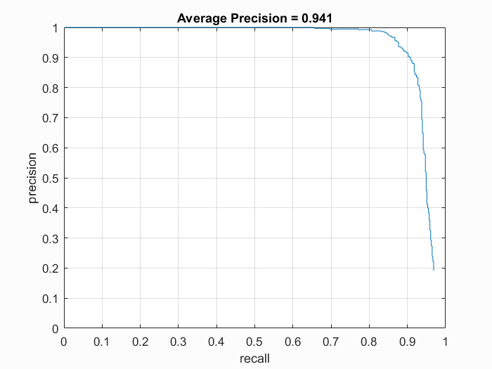
We seem to have achieved very similar performance to Viola Jones.

We will now look at our two top performing face detectors. On the left, we have our face detector that did not use hard negatives (93.9%) and on the right, we have our face detector that did use hard negatives (94.1%). It starts to become clear that we end up with less false positives with the hard negative mining (both detectors only kept predictions that has SVM responses greater than -0.2).

Conclusion

Thanks to the work of Dalal and Triggs, we can detect faces at reasonable accuracy with relatively little complexity. This project really highlights the power of SVMs and image features such as HOG. These well established black boxes leave us with little additional effort required to solve a seemingly difficult task. In this application, hard negative mining appears to impove the quality of our face detections by removing false positives, but does not tend to improve precision at such high performance already. This could be a more useful technique if we had less data to train on.