Project 5 / Face Detection with a Sliding Window
Overview
For this project, a Dalal-Triggs style sliding window face detection algorithm was implemented in Matlab. This detector first acquired a set of positive training examples of faces and a set of negative training examples sampled randomly from images with no faces. Each of these examples was converted to Histogram of Oriented Gradients (HOG) feature space. The detector then trained a linear Support Vector Machine (SVM) classifier on these training examples. To detect faces in new images, the SVM was applied using a sliding window at multiple scales for each image. To improve the performace of the SVM classifier, the SVM was applied to the set of non-face training images and the hard negative face detections produced were used to retrain the SVM. The resulting accuracy was 81.1% without hard negative mining and 84% with hard negative mining.
Implementation
The first step of the algorithm is to get HOG features for each of the positive and negative training examples. The following code (get_positive_features()) shows how each of the positive examples is created:
image_files = dir( fullfile( train_path_pos, '*.jpg') );
num_images = length(image_files);

features_pos = zeros(num_images, (feature_params.template_size / feature_params.hog_cell_size)^2 * 31);
for i = 1:num_images
    img = imread(fullfile(train_path_pos, image_files(i).name));
    hog = vl_hog(im2single(img), feature_params.hog_cell_size);
    features_pos(i,:) = reshape(hog, [1, (feature_params.template_size / feature_params.hog_cell_size)^2 * 31]);
end
Each of the input images is a 36x36 image of a face. Each image is read in, converted to HOG space using VLFeat's vl_hog() function, and flattened into a single feature vector. The negative training examples are created in a similar way in get_random_negative_features():
image_files = dir( fullfile( non_face_scn_path, '*.jpg' ));
num_images = length(image_files);
samples_per_img = floor(num_samples / num_images);

features_neg = zeros(num_samples, (feature_params.template_size / feature_params.hog_cell_size)^2 * 31);
for i = 1:num_images
    img = rgb2gray(imread(fullfile(non_face_scn_path, image_files(i).name)));
    for j = 1:samples_per_img
        % Scale image randomly from 1/2 to 1.5 times size
        scale = rand() + max(0.5, feature_params.template_size / min(size(img) + 0.01));
        ims = imresize(img, scale);

        % Crop image randomly
        x = randi(size(ims, 2) - feature_params.template_size);
        y = randi(size(ims, 1) - feature_params.template_size);
        imc = imcrop(ims, [x, y, feature_params.template_size, feature_params.template_size]);

        % Get HOG features
        hog = vl_hog(im2single(imc), feature_params.hog_cell_size);
        features_neg((i-1)*j+j,:) = reshape(hog, [1, (feature_params.template_size / feature_params.hog_cell_size)^2 * 31]);
    end
end
For the negative feature extraction, each image is scaled randomly and then cropped at a random location with size 36x36 before converting to HOG space. This is done multiple times for each image to produce a large number of negative examples. The total number of random negative samples used was 100000 as this produced a high accuracy while taking only a few minutes to compute. Once the positive and negative features have been computed, the SVM classifier is trained on these examples (proj_5.m):
lambda = 0.001;
[w, b] = vl_svmtrain([features_pos; features_neg]', [ones(1, size(features_pos, 1)), -ones(1, size(features_neg, 1))], lambda);)
The lambda value chosen for the SVM was 0.001 because this value yielded the highest precision. The resulting SVM classifier can then be applied as a sliding window to each test image to produce face detections, as shown in run_detector() below:
test_scenes = dir( fullfile( test_scn_path, '*.jpg' ));

%initialize these as empty and incrementally expand them.
bboxes = zeros(0,4);
confidences = zeros(0,1);
image_ids = cell(0,1);

% Run on each image
for i = 1:length(test_scenes)

    fprintf('Detecting faces in %s\n', test_scenes(i).name)
    img = imread( fullfile( test_scn_path, test_scenes(i).name ));
    img = single(img)/255;
    if(size(img,3) > 1)
        img = rgb2gray(img);
    end

    curr_bboxes = zeros(0,4);
    curr_confidences = zeros(0,1);
    curr_image_ids = cell(0,1);

    % For each image, run sliding window at multiple scales
    for scale = 0.2:0.01:1.2
        % Scale and get HOG representation
        ims = imresize(img, scale);
        imshog = vl_hog(im2single(ims), feature_params.hog_cell_size);

        % Run sliding window at step size equal to half the size of the HOG
        % window
        for j = 1:feature_params.template_size/feature_params.hog_cell_size/2:size(imshog, 1)-feature_params.template_size/feature_params.hog_cell_size
            for k = 1:feature_params.template_size/feature_params.hog_cell_size/2:size(imshog, 2)-feature_params.template_size/feature_params.hog_cell_size
                % Get subimage and run SVM
                subimg = imshog(j:j-1+feature_params.template_size/feature_params.hog_cell_size, k:k-1+feature_params.template_size/feature_params.hog_cell_size, :);
                pred_label = w'*reshape(subimg, [(feature_params.template_size / feature_params.hog_cell_size)^2 * 31, 1]) + b;

                % Label as a face if confidence is above a threshold
                if pred_label > -1.5
                    x = (k-1)*feature_params.hog_cell_size+1;
                    y = (j-1)*feature_params.hog_cell_size+1;
                    curr_bboxes = [curr_bboxes; [floor(x/scale), floor(y/scale), floor((x+feature_params.template_size)/scale), floor((y+feature_params.template_size)/scale)]];
                    curr_confidences = [curr_confidences; pred_label];
                    curr_image_ids = [curr_image_ids; test_scenes(i).name];
                end
            end
        end
    end

    % Non-max suppression
    [is_maximum] = non_max_supr_bbox(curr_bboxes, curr_confidences, size(img));
    curr_bboxes = curr_bboxes(is_maximum,:);
    curr_confidences = curr_confidences(is_maximum);
    curr_image_ids = curr_image_ids(is_maximum);

    bboxes      = [bboxes;      curr_bboxes];
    confidences = [confidences; curr_confidences];
    image_ids   = [image_ids;   curr_image_ids];

end
Each testing image is scaled at increments of 0.01 from 0.2 times the original size to 1.2 times the original size. These values were tuned manually to produce the highest precision. After the image is scaled, it is converted to HOG space using vl_hog(). A sliding window is then applied to the HOG representation of the image. This window is computed at increments of half the size of the HOG window. A smaller step size will tend to yield better precision, but will take longer to compute. Choosing half the window size appeared to be a good tradeoff in testing. Each window is then classified with the SVM. If the SVM output is greater than -1.5, it is labeled as a face. This threshold is quite low, so it will tend to produce a large number of false positives, but will avoid missing too many true positives. Finally, non-maximum suppression is used to prevent duplicate detections.
To further improve the detection results, hard negative mining is implemented using the code below from proj_5.m:
% Run detector on non-face images
[bboxhn, conhn, idhn] = run_detector(non_face_scn_path, w, b, feature_params);

% Sort by confidence and take the top 5000 false positives
[~, idx] = sort(conhn, 'descend');
hns = zeros(min(5000, length(conhn)), (feature_params.template_size / feature_params.hog_cell_size)^2 * 31);
for i = 1:min(5000, length(conhn))
    bbox = bboxhn(idx(i), :);
    img = rgb2gray(imread(fullfile(non_face_scn_path, idhn{idx(i)})));

    % Handle bounding boxes not completely contained in the image
    if bbox(2) < 1
        bbox(4) = bbox(4)+abs(bbox(2))+1;
        bbox(2) = 1;
    end
    if bbox(1) < 1
        bbox(3) = bbox(1)+abs(bbox(1))+1;
        bbox(1) = 1;
    end
    if bbox(4) > size(img, 1)
        bbox(2) = bbox(2)-bbox(4)+size(img, 1);
        bbox(4) = size(img, 1);
    end
    if bbox(3) > size(img, 2)
        bbox(1) = bbox(1)-bbox(3)+size(img, 2);
        bbox(3) = size(img, 2);
    end

    % Convert to HOG space
    subimg = imresize(img(bbox(2):bbox(4), bbox(1):bbox(3)), [feature_params.template_size, feature_params.template_size]);
    hog = vl_hog(im2single(subimg), feature_params.hog_cell_size);
    hns(i,:) = reshape(hog, [1, (feature_params.template_size / feature_params.hog_cell_size)^2 * 31]);
end

% Retrain svm with hard negatives
[w, b] = vl_svmtrain([features_pos; hns]', [ones(1, size(features_pos, 1)), -ones(1, size(hns, 1))], lambda);
The hard negative examples are found by running the detector on the non-face training images. The resulting detections are sorted by confidence, and the top 5000 false positives are chosen as the hard negative examples. These are converted to HOG space and the SVM is retrained with the hard negatives.
Results
The detection algorithm was run on the test set both with and without hard negative mining to compare the results. The images below show the precision/recall curves and a sample detection output for each case (HOG cell size of 6):
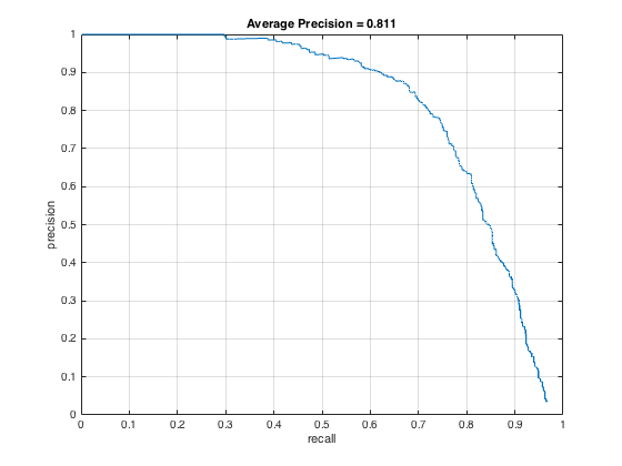
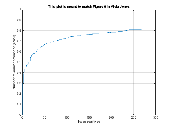
Precision/recall curves for detection (no hard negative mining).
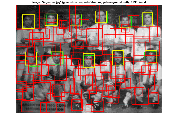
Detection output (no hard negative mining).
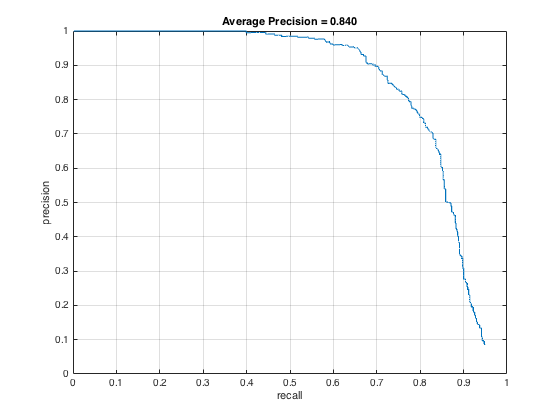
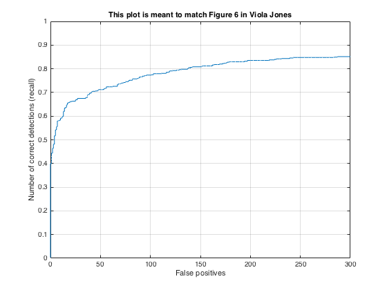
Precision/recall curves for detection with hard negative mining.
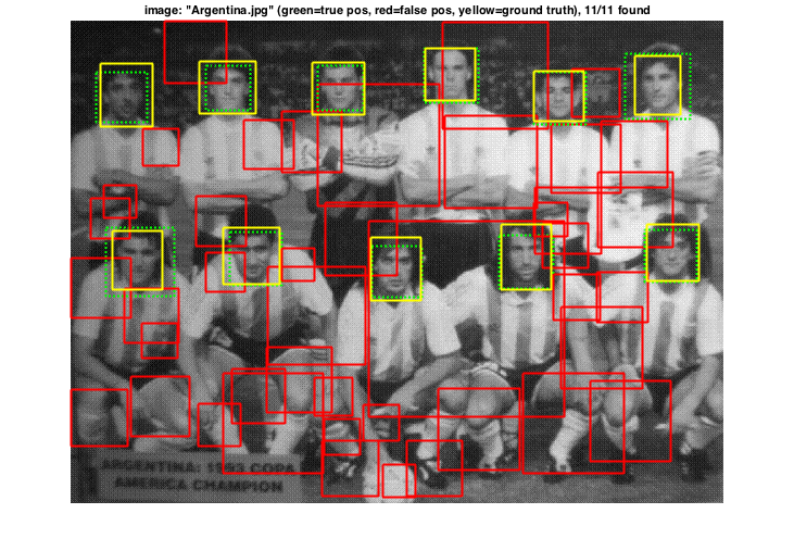
Detection output with hard negative mining.
The average precision for the detection without hard negative mining was 81.1%. This value fluctuates somewhat depending on the randomness of the negative training samples. By running hard negative mining, the average precision increased to 84%. In both cases, all faces were detected in the sample image shown, but the hard negative mining produced fewer false positives. By limiting the number of high confidence false positives, the average precision can be improved. The images below show examples of face detections on two images of the class:
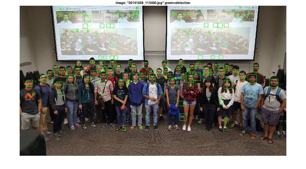
Front face detection of the class.
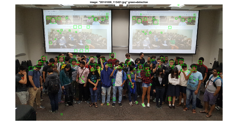
Hard face detection of the class.
The first class photo is much easier to detect because most of the faces are forward facing. The faces the detector misses are those that are partially occluded, rotated sideways, or are faces that are difficult to see on the projector. In the second image, only a few faces can be detected successfully since almost all of the faces are turned or partially occluded.