Project 5 / Face Detection with a Sliding Window
The goal of this project was to implement a face detector using the sliding window detector of Dalal and Triggs. This was achieved in four main steps:
- Load cropped positive training examples
- Randomly sample negative examples
- Train a linear classifier from the positive and negative examples
- Run the classifier on the set of test images
Loading Positive Training Examples
This step was simply a matter of going through the CalTech face database and transforming each image into a histogram of oriented gradients (HOG). These HOG representations of positive training examples were used as positive features train the linear classifier.
Randomly Sampling Negative Examples
Getting negative training examples was also reasonably straightforward. Until an arbitrary number of negative examples was reached, an image was randomly selected from the set of non-face scenes, the image was then randomly scaled, and a window of the same size as the HOG template was randomly cropped from the image. Finally, these cropped windows were transformed into HOG representations, like the positive training examples, and used as negative features for the linear classifier.
Training the Linear Classifier
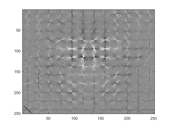
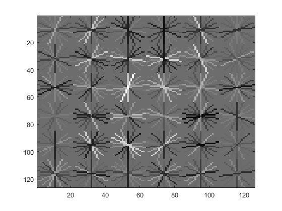
Using the collected positive and negative training examples, a support vector machine (SVM) was trained with VLFeat's vl_svmtrain function. The result is the learned face detector, visualized below.
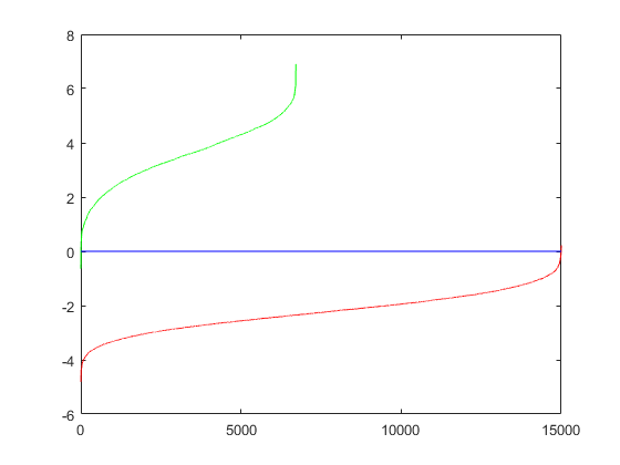
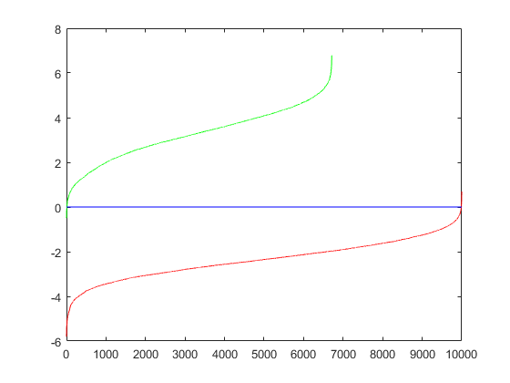
Furthermore, to ensure the positive and negative training examples are sufficiently different, their separation can also be visualized where the green line represents positive examples and the red line represents negative examples.
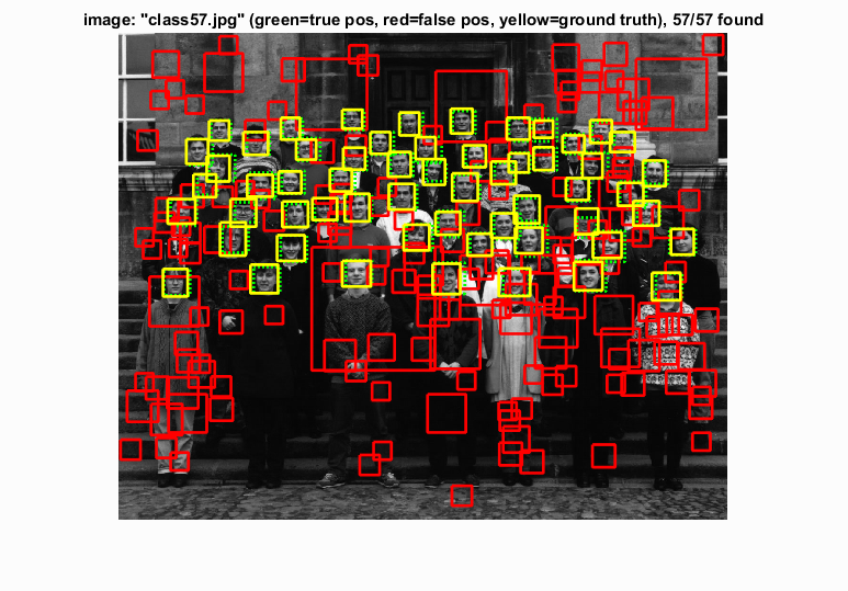
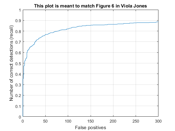
Running the Classifier on Test Images
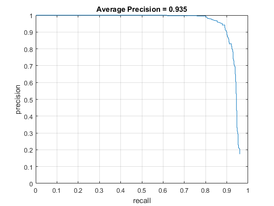
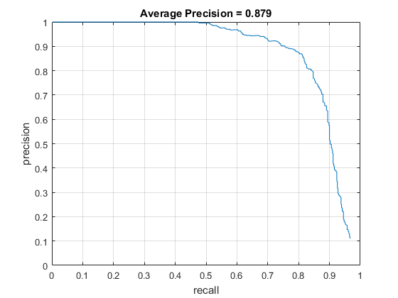
Finally, the learned face detector was run against images in the set of test images. For a range of scales in each image, the image was transformed into a HOG representation and divided into cells on which the sliding window would operate on. The HOG features would be extracted from the sliding window at each cell and used to compute a confidence score for each cell. All cells whose confidences were above a certain threshold were determined to contain a face. A bounding box for each of these positive cells was saved, along with their confidence, and image ID for evaluation. The evaluation then determines the average precision of the face detector based on ground truth values in the test set.
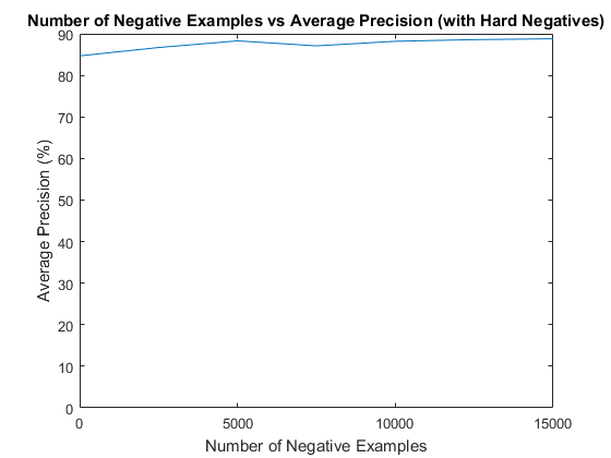
Mining Hard Negatives
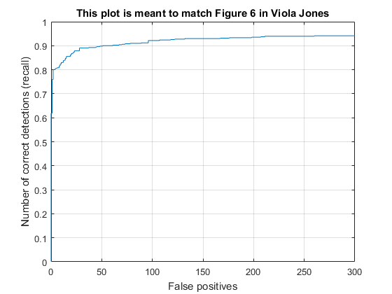
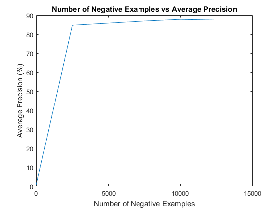
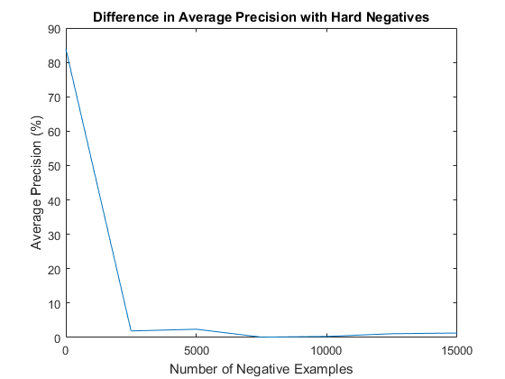
In addition to the randomly sampled negative training examples, an attempt at mining for hard negatives was also made. Before running the classifier on the test images, it was run on the set of non-face scenes to find areas that it believed contains faces. The results of this are rigged to contain only false positives, so this additional negative examples were then used to retrain the classifier before finally running the classifier against the actual test set of images. Unfortunately, mining for hard negatives did not show a significant improvement in average precision with the default parameters. Specifically, with a large number of randomly sampled negative examples, the addition of hard negatives showed only negligible improvement. However, with a more limited set of randomly sampled negative examples (less than 5000), there was significant improvement. Particularly, in the complete absence of the randomly sampled negative examples, the use hard negatives was more or less able to compensate.
Parameter Tuning
All the figures listed above were assumed to be using the default given parameters, with the exception of the threshold parameter when running the classifier because it was not a given value. A threshold of -0.1 was used because it was found to be optimal over a range of values.
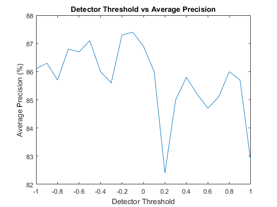
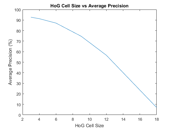
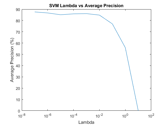
Threshold aside, there were four other parameters to test (HOG cell size, number of randomly sampled negative examples, whether or not hard negatives were used, and λ), so each one was tested independently with a threshold of -0.1 and default values where applicable.
HOG cell size was the most significant parameter in affecting average precision. Smaller cell sizes were strictly better, but drastically increased memory usage and runtime. Cell sizes of 1 and 2 were attempted, but my system did not have enough memory to complete the pipeline.
The results for varying the number of randomly sampled negatives examples and the use of hard negatives were displayed above in the section on mining hard negatives, but it appears that more negative examples performed strictly better, though not by much beyond 10,000.
In using vl_svmtrain, there is a regularization parameter λ that can be adjusted. λ did not appear to have a significant impact on the average precision unless it was greater than 0.01, but smaller values seemed to perform better.
Results of combining the best values for each parameter
HOG Cell size = 3, 15000 randomly sampled negative examples, hard negatives, λ = 0.0000001, threshold = -0.1