Project 5 / Face Detection with a Sliding Window
The task to be accomplished for project 5 was to detect faces in a given set of test images by training the machine via SVM with positive and negative features of faces and using a detector to compare features of faces & non-faces to the train data. The sliding window model was used to collect and detect features generated by the Histogram of Gradient (HoG) representation. The windows of features were taken at multiple scales for scale-invariance of the implementation. The tasks for the project assignment can be divided into 5 parts (including the graduate credit task):
- Get positive features from training data.
- Get random negative features from training data.
- Train the SVM classifier using collected features and corresponding labels.
- Design detector to find faces in test data using the SVM classifier.
- Implement hard negative mining on the SVM classifier (graduate credit).
Collecting Positive Features
Positive features from training images of faces provided by Caltech were collected by calculating HoG from each image and saving them in the feature variable. The parameter to change was the size of each cell of the HoG (hog_cell_size). The smaller the cell size is, the better is the accuracy of the detector, but with slower runtime. The attempted cell sizes were 6, 4, and 3 pixels respectively, but the ultimately chosen cell size was 6 pixels, as the accuracy gain was ~5% (gain from 85% to 95%) with 10~15 min. increase in runtime, which I considered to be too costly for the accuracy gain of roughly 5%.
Collecting Random Negative Features
Negative features from training images of non-faces were collected by similar principles with collecting positive features; however, instead of taking the HoG of the whole image, random templates of the image were taken for capturing negative features. The number of features to take from each image was determined by a pre-determined parameter num_samples, and diving it by the number of images (and rounding it down). The parameters to change in this task were the template_size, hog_cell_size, and the num_samples. The template size was to be divisible by hog_cell_size as each template was built up by groups of cells. Since the detector to be implemented is to apply downscaling of images to avoid complexity, the template had to be big enough to capture the wide range of scales. template_size provided by the starter code was 36 pixels, which seemed to work fine with the majority of scales, so it was left as is. hog_cell_size was chosen as 6 pixels as before for consistency. num_samples, or the number of total samples to take was chosen as 10000. The number 5000 was chosen as alternative for comparison, but this resulted in providing a higher number of false positives, thus decreasing the accuracy of the detector. Using 20000 samples increased computation time by 5~10 min. but only increaseing accuracy by ~0.5%, thus 10000 samples were taken from negative data.
Training SVM classifier
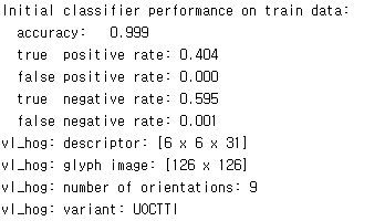
Training the SVM classifier was accomplished by concatenating the positive features and the negative features, and labeling them with appropriate logics (1 for positive, -1 for negative). The regularization parameter for the SVM classifier, lambda, was chosen as 0.0001 as suggested by the starter code; other values weren't tested, but changing it could overfit, underfit data if it were to be tweaked significantly. Then, all the values mentioned above were trained using the vl_svmtrain function provided by VLFeat. The results of the classifier can be seen below:
Classifier performance
Face Detection
Face detection was accomplished by taking each test data and utilizing the sliding window technique to trace through the image by shifting the window by each cell unit (6 pixels as determined above) and scoring each window using the w and b values determined by the classifier above. The windows with scores higher than a given threshold was to be determined as faces in that image. For scale invariance, windows were taken with differing scales of the same image. Then, for each image, non-maximum suppression was implemented in order to avoid repetitive representation. The important parameters considered in this task were: threshold for scoring each window, and scale range to take from each image. The threshold score for detecting faces was chosen as 0.5, simply because it gave the best performance. Other threshold values attempted were 0.75 and 0.85. Values lower than 0.5 just gave too many false positives, and threshold values of 0.75 and 0.85 gave fair results, but in some cases the detector was too strict and neglected features that were actually positive for faces. The scale range for testing each window was chosen from 1, the original size, to 0.1 times the original, with decreasing step size of 0.1 (so it would be 1, 0.9, 0.8,..., 0.1). More scale values in between would provide more accurate results, and scale values lower than 0.1 would enable detection of larger features, but this range was chose due to optimal computation time and adequate inclusiveness of test features. The results of implementing face detector can be seen below.
Face template HoG visualization.
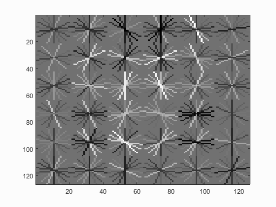
It can be seen that the HoG visualization somewhat resembles that of a human face.
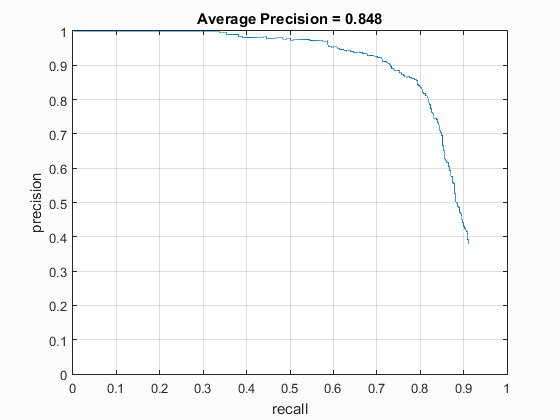
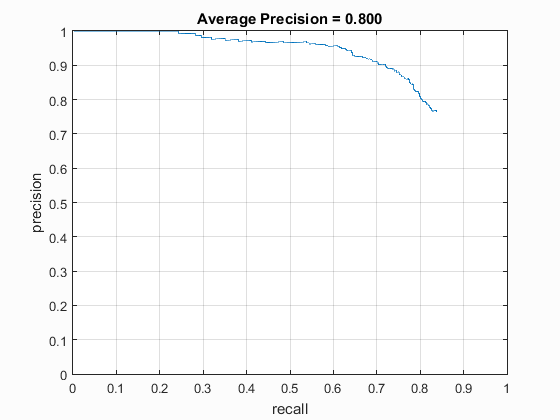
Precision Recall curve for detection with random negatives.
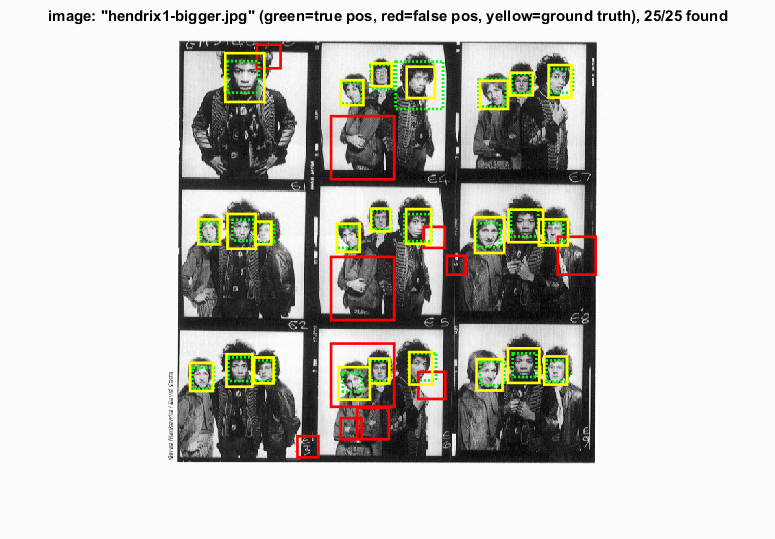
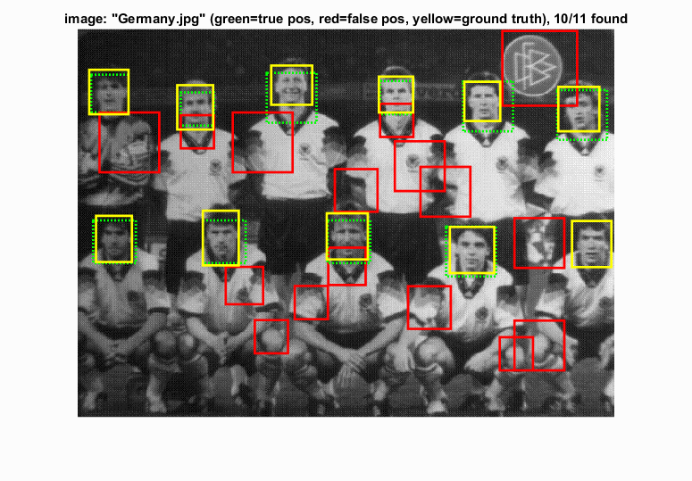
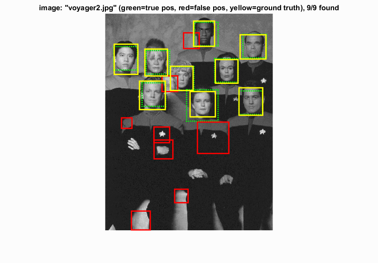
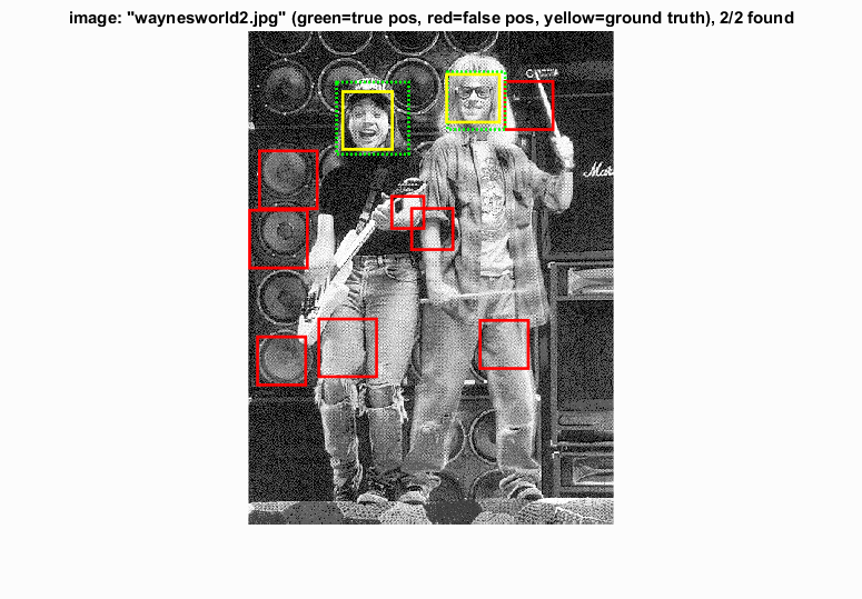
Example of detection on the test set.
Hard Negative Mining (graduate credit)
Hard negative mining was accomplished by using the detector mentioned above and collecting the false positive features from the pool of non-face images and adding them to the pool of features for training the SVM classifier. Implementing hard mining resulted in neglection of a good amount of false positive, where at the same time neglecting some of the true positives. The parameters that were used in this tasks were threshold for scoring features and number of samples to take from false positives. The threshold value was chosen was 0.5, same as for using the detector to find positive faces. Values higher than 0.5 (0.75 was tested) resulted in less significant change in the detection. Values lower than 0.5 resulted in neglecting not only a large amount of false positive features, but also a good amount of true positives. The change number of samples of false positives resulted in a simular fashion, larger number neglected more features, smaller number neglected less. The results of implementing hard negative mining can be seen below.
Precision Recall curve detection with hard negative mining.
Comparison of results of detection with random negatives and with hard negative mining.
Detection with random negatives
Detection with hard negative mining
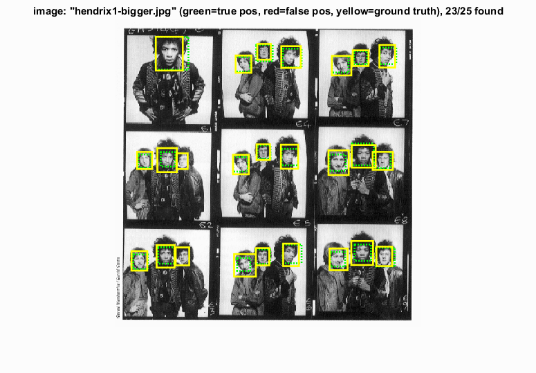
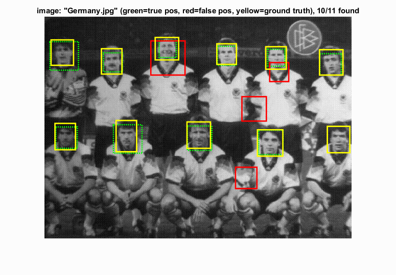
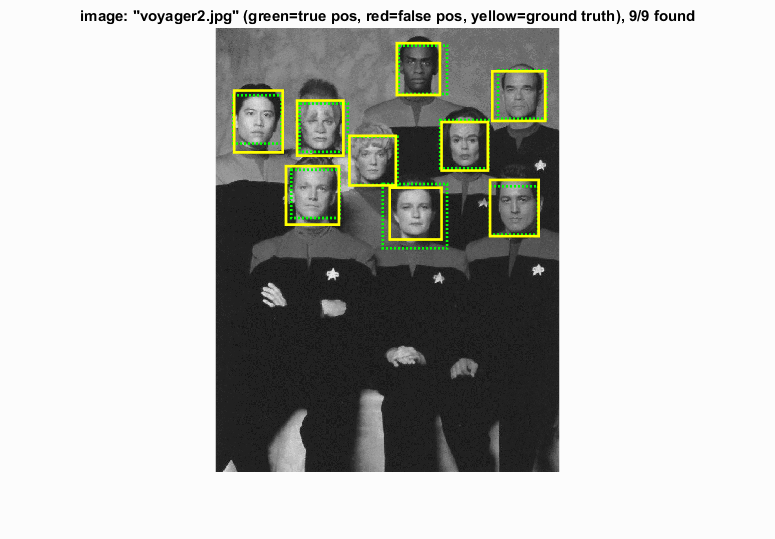
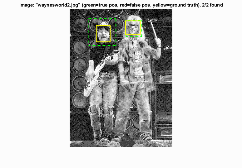
It can be seen from the precision vs. recall curve and the example test images that implementation of hard mining may decrease the accuracy of the detection overall, but it also alleviates extraneous detection of false positives as it can be clearly seen in the examples.