Project 5 / Face Detection with a Sliding Window
Overview
For this project, we had to create a mutli-scale, sliding window face detector. The detector uses HoG features to train a linear SVM. The following is the steps to complete this project
- Obtaining positive and negative traing data
- Training a linear SVM
- Running the detactor on the test set
- Visualization of results
Extra credits:
- Hard negative mining
- KNN
Obtaining Training Data
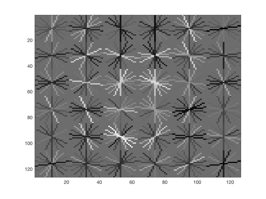
The positive examples are presented and pre-cropped, whereas the negative examples need to be randomly selected and cut the same siz as the positive examples from non-face set. All positive and negative images are converted to HoG space as a sample in the feature matrix. In the experiment, we use template size = 36, hog_cell size = 6, then we get 6713 positive samples, and 9937 negative samples.
Training the SVM
All windows are converted to HoG space and are marked as either being face/non-face. We can mark all our negative examples as non-face because we know that no faces appear in the images they were obtained from, so there is no possibility of cropping out a face. VL_Feat is used to obtain the weights and offsets for the linear SVM, with lambda = 0.0001. Test results show that the accuracy of linear SVM achieves 0.999.
Running the Detector
The image is converted to HoG space and a sliding window the size of the template is moved across the hog space. The confidence of each window is calculated, the bounding box is recorded and added as a potentional max. The image is then resized and the process continues until the image is smaller than the template. Having a larger (closer to 1) scale factor increases performance as it is finer steps in face size. This is at the cost of many more passes of the sliding window in the construction of the image pyramid.
Non-maxima suppression is run on all the bounding boxes at all scales to find the most confident box and eliminate detection at multiple scales / the same location.
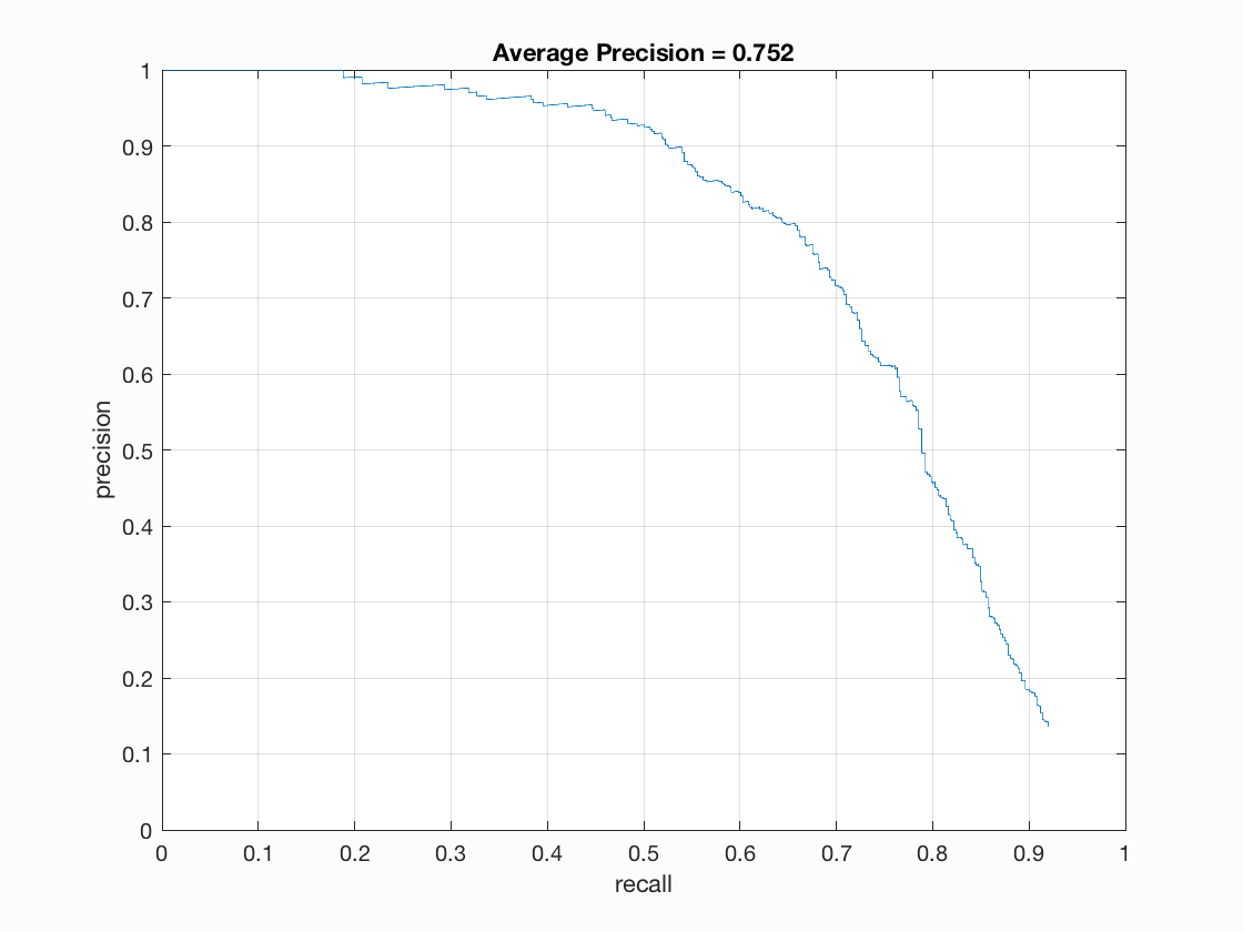
Multiple scales greatly improved the performance of my detector. The single scale performed poorly at only around 40% average precision. Implementing multiple scales greatly improved prevciosin, bringing it up to 75.2%.
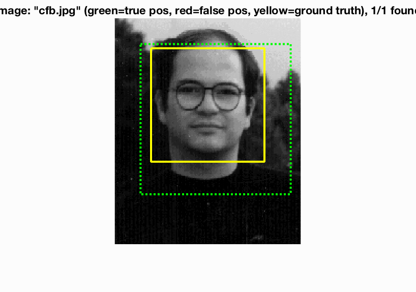
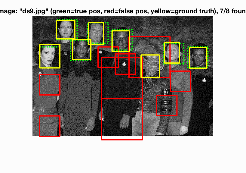
Sample Results
|
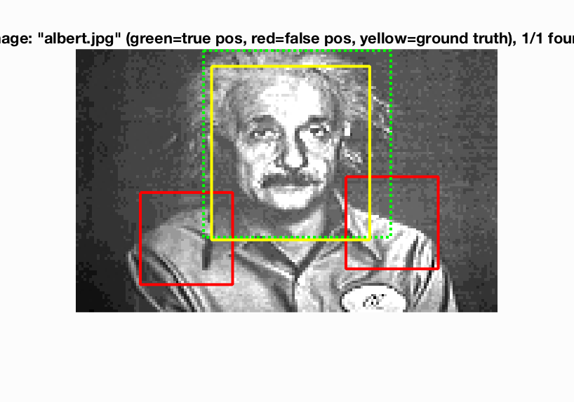
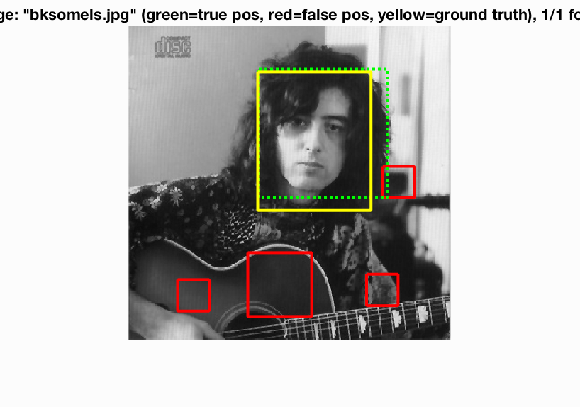
|
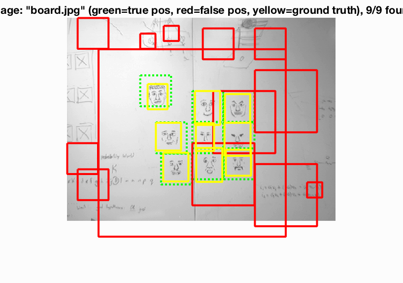
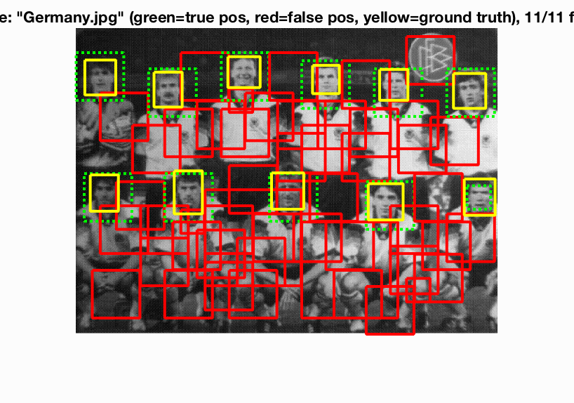
|
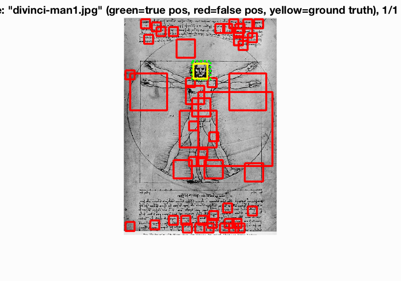
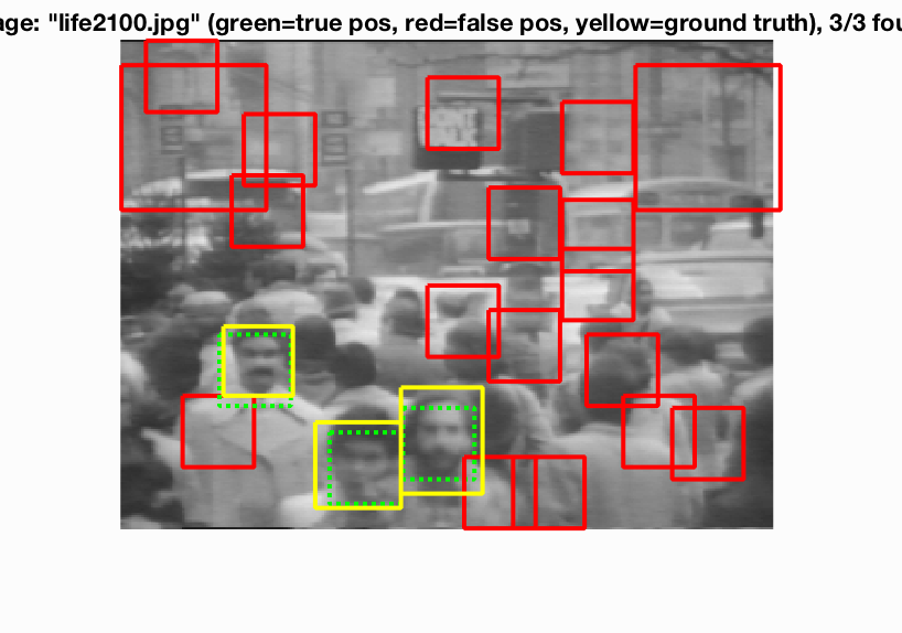
|
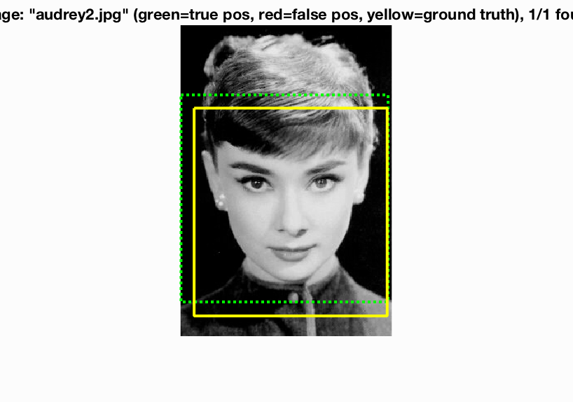
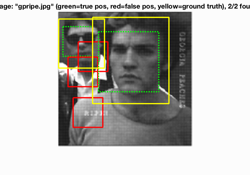
|
Precision Recall curve for the multi-scale-detector with step size of 6.
Extra Credits
Hard negative mining
Run the detecor on the non-face data set using trained linear SVM, to mine the negative features which are hard to distinguish. Append all the false positive features to the feature matrix, and train the linear SVM again using the updated feature matrix and labels. Then we can apply this classifier on our test data. Threshold for hard mining is theta = =-0.5, for detector is theta = -1, lambda in SVM is 0.0001, template size = 36, hog_cell size = 6. After hard negative mining, we achieve avg. accuracy = 76.0%, nearly 1% increment.
.png)
KNN
We implement a KNN classifier in the detector. If the feature matrix has number of samples > 300, we do a dimension reduction to dim = 20 using PCA. To calculate the confidence, we using weights as the reciprocal of the distance, and compute the confidence of each test sample as the weighted mean of the labels of K nearest neighbors. Thrshold is 0.9, since most of the possible samples have confidence = 1. KNN classifier is very time consuming, I used 52 mins to get accuracy = 8%. The low accuracy results from too many false positive. So we need to have better weights to generate more divergent confidence, then we can distinguish false positive better.
.png)