Project 5 / Face Detection with a Sliding Window
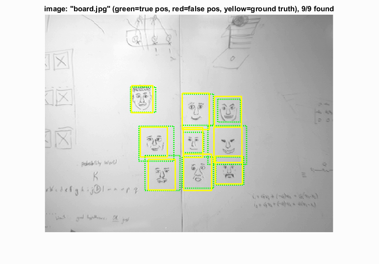
Example output of the face detector.
- Create positive feature examples from a set of cropped face images.
- Mine a set of images with no faces to create a set of a specific size holding negative feature examples
- Train a (linear support vector machine) classifier on the set of features and their labels. The label set is {-1, 1}, where -1 is negative and 1 is positive.
- Run the sliding window detector on a set of test images that have ground truth labels, and compute precision, recall, and other metrics.
Implementation details
The positive HOG features were built from cropped images of faces, each of which was 36 x 36 pixels. These images were sectioned into smaller groups called cells, for example 6x6, and then the histogram of gradients was computed for each cell, as visualized below. Each cell holds 31 data points, and each feature vector was "flattened" into a 1-D vector, which had 1116 entries in the 6x6 cell case.
Negative HOG features were computed in the same way as the positive HOG features, except that larger images were used, and random sections of 36x36 pixels were used to build features. Images were randomly sampled with replacement, and 10 features were extracted from random windows within each randomly sampled image, until the specified number of negative examples was reached.
The features were then concatenated, and I used a linear SVM to find the vectors w and b that define the hyperplane the attempts to separate face from non-face examples in feature space. The regularization parameter lambda was set to 0.0001 and not changed for this project.
Finally, the sliding window detector was used to find faces in new images. The image was rescaled (shrunk) several times until it was smaller than the template size, which ensured that all ranges of face sizes could be searched for. At each scale, the HOG features were computed for every possible window corresponding to the same feature size as the training examples. Then, using the w and b vectors, I calculated the confidence that each window was a face, and thresholded it as an initial filter. Finally, non-maximum suppression was performed on the set of possible faces to distill them to a single prediction.
The parameters I chose to tweak for this project were the number of negatives sampled and the threshold on face detection. Below is a portion of the code I wrote for the sliding window detection.
while scale*size(img,1) > feature_params.template_size && scale*size(img,2) > feature_params.template_size
    imscaled = imresize(img,scale);
    imhog = vl_hog(imscaled, test_cell_size);
    %sliding window
    for x = 1:size(imhog,2)-num_hog_regions+1
        for y = 1:size(imhog,1)-num_hog_regions+1
            window = imhog(y:y+num_hog_regions-1,x:x+num_hog_regions-1,:);
            feature = reshape(window, (num_hog_regions^2) * 31, 1);
            confidence = w'*feature + b;
            if confidence > threshold
                %face detected
                num = num + 1;
                %get the coordinates of the box and save them
                x_min = floor((1 + (x-1)*test_cell_size)/scale);
                y_min = floor((1 + (y-1)*test_cell_size)/scale);
                %maxes are the mins plus template size, scaled, but not
                %out of bounds
                x_max = floor((x_min + num_hog_regions*test_cell_size/scale));
                y_max = floor((y_min + feature_params.template_size/scale));
                cur_bboxes(end+1,:) = [x_min, y_min, x_max, y_max];
                cur_confidences(end+1,1) = confidence;
                cur_image_ids{end+1} = test_scenes(i).name;
            end
        end
    end
    scale = scale * 0.9;
end
The scale factor was set to 0.9 after smaller values were found to be too coarse.
Results in a table
The results below are using 10k negative samples and a threshold of 0.1 on the left, and 50k negative samples with a threshold of 0.5 on the right. I had noticed that the number of false positives seemed too high in the initial (left) configuration, so I sampled more negative features. Then I had to lower the threshold a bit to make up for it, which ended up causing lower average precision. It's possible the greater number of negative features could be more accurate if the thresholding and other parameters were explored further. For these examples, a 6x6 cell size was used.
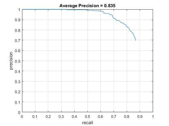
We can see that the left curve is strictly better: for a given precision, its recall is higher, and for a given recall, its precision is higher. |
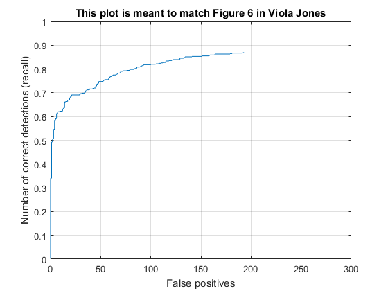
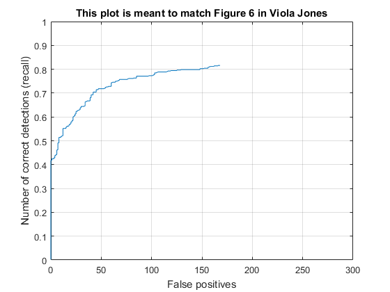
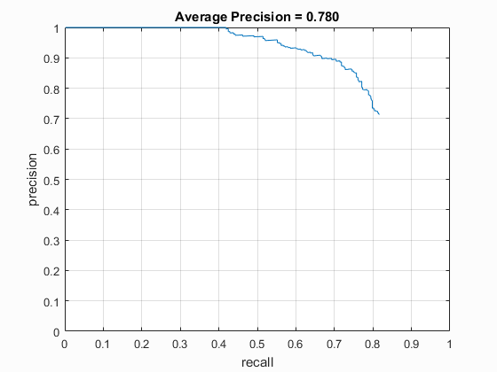
Similar to the above, both resemble the figure from the original Viola Jones paper, however for the same number of false positives, the left example has higher recall. The right example shows that it has less false positives overall. |
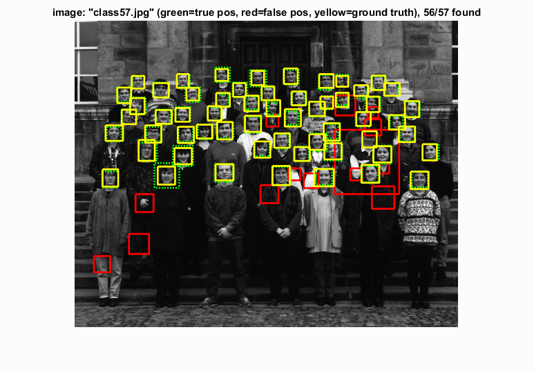
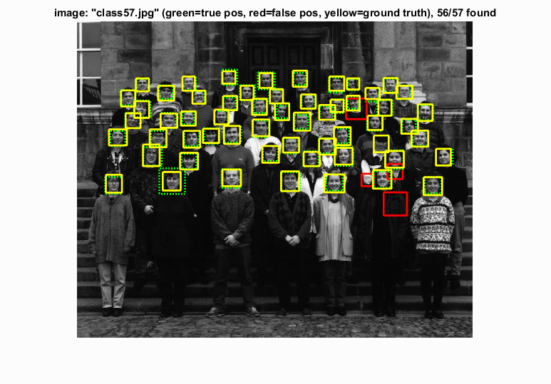
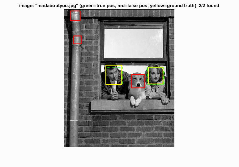
An example that shows how the right configuration did reduce the number of false positives and improve accuracy (in this case). The same number of true positives is detected in both images. |
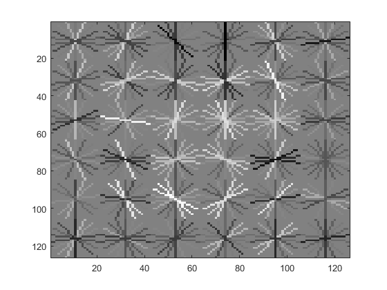
Left: the feature visualization (a 6x6 grid of cells, each one 6x6 pixels) for the left configuration. Right: An example showing how non-human faces could be accidentally detected by this detector. |
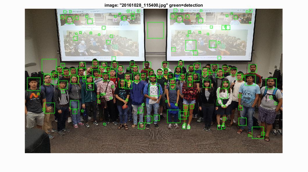
Performance on this year's "easy" picture. The detector was able to pick up some of the faces on the projector screen as well, but the amount of falsep positives is relatively high.
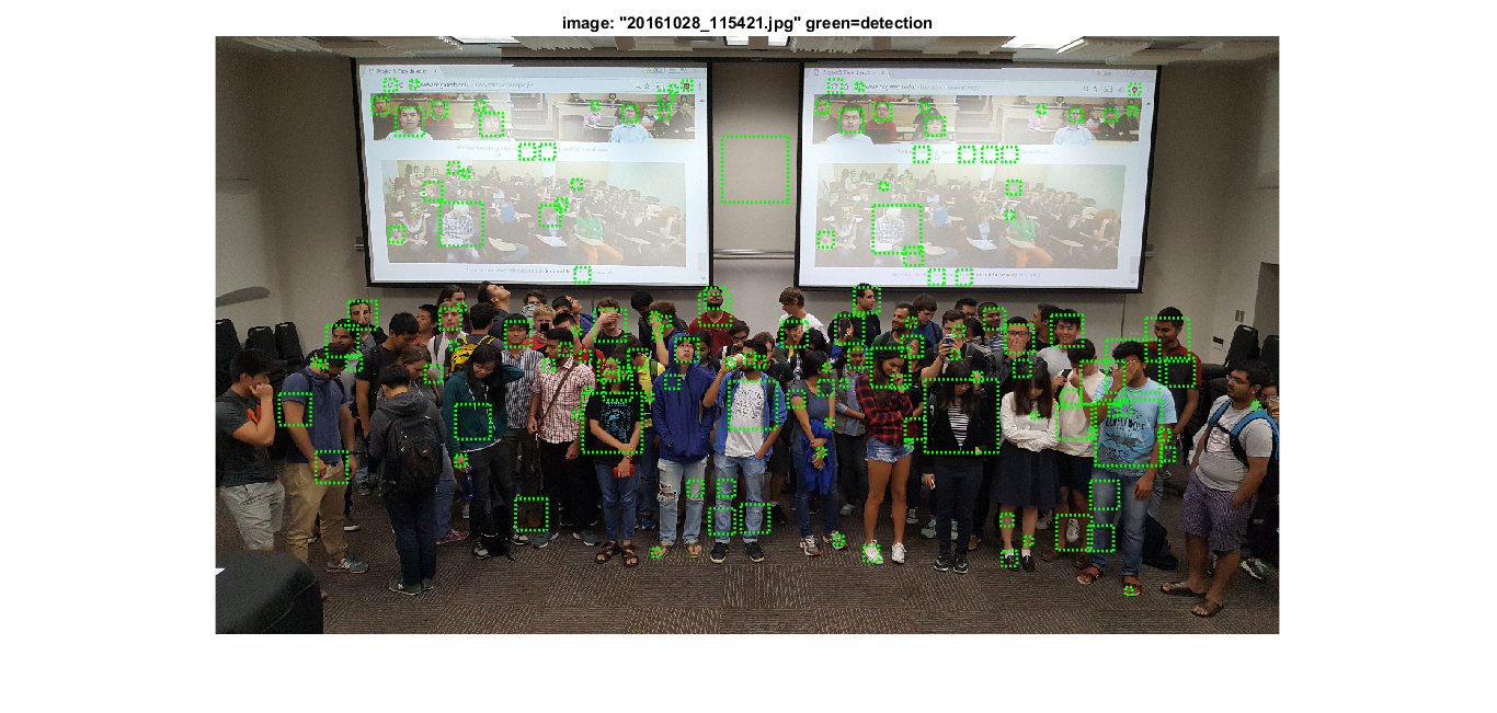
Similarly, some faces are detected, but the precision is low.
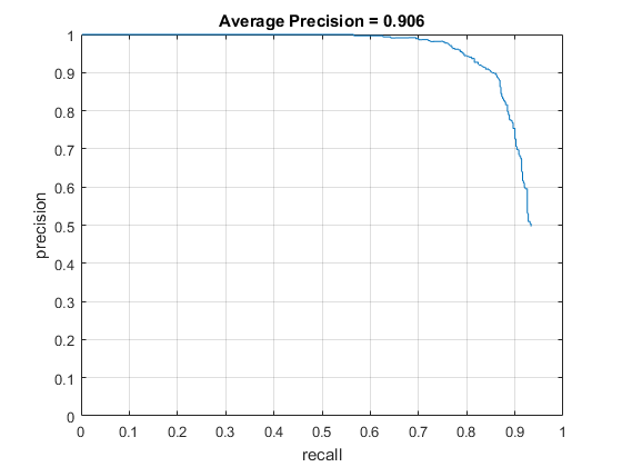
I also ran the detection pipeline with threshold 0.5, 50k negative samples, and changing the cell size to 4x4 pixels. This increased the average precision up to 90.6%, as shown below. The average precision is much higher, but the overall minimum precision is lower, meaning more false positives were recorded.