Project 5 / Face Detection with a Sliding Window
The objective of this project is to develop a face detection program by implementing the sliding window detector of Dalal and Triggs 2005. The algorithm primarily includes the following steps.
- Develop Histogram of Gradients (HOG) features for negative and positive face example;
- Train a linear support vector machine (SVM) based on the negative and positive HOG features;
- Detect potential faces by sliding windows at varying locations with different image scales;
- Conduct non-maxima suppression on the detected faces in each image.
The highest average precision achieved by this program is 0.913 using a step size of 3 and downsample scale of 0.9. Different HOG cell and sliding window step sizes, downsample scales, and confidence thresholds will be tested to compare different performances. An extra positive examples are also tested for extra credits.
Implementation
Basic Setting
The positive training database is 6,713 cropped 36x36 face images from the Caltech Web Faces project. The negative training database is generated by randomly sampling 10,000 cropped 36x36 non-face images from Wu et al. and the SUN scene database. The scenes are also randomly scaled between one to three during sampling to generate rich negative training database. The HOG descriptor for each cropped image is generated using the vl_hog function, which divides each cropped image into 6x6 cells and generate a 6x6x31 dimension descriptor for each image. The step size of the sliding window is set to be the same as the cell size. The Lambda for SVM classifier is 0.0001 and confidence threshold is set as 0.5 by default.
Version 1
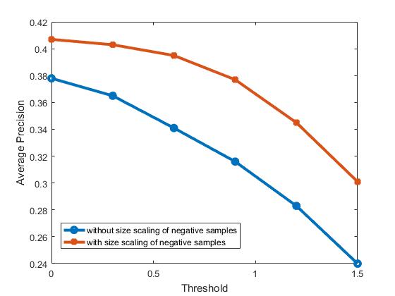
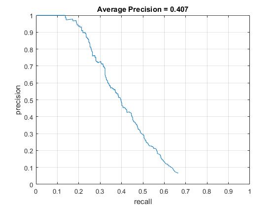
In the first version, the potential faces in each test image are detected without image downsample. Therefore, only the face with a size about 36x36 can be detected because the all training examples have the size of 36x36. Since the number of negative scenes are limited, I have also tested the detection performance by randomly scaling (between one to three) the negative scenes. Besides, different confidence thresholds (0, 0.3, 0.6, 0.9, 1.2, and 1.5) are tested to see their effects on the detection precision. The test results are shown in the first image below. The highest average precision about 0.407 is achieved when threshold is 0 and negative scene scaling is implemented. Therefore, I will 0 as the threshold and negative scene scaling to improve the average precision. The training time with and without negative scene scaling is about 243s and 295s, respectively. The testing time for all cases are around 90s. The visualization of the learned classifier, precision recall curve, and the results of some test images are shown as follows.
Precision comparison with different thresholds.
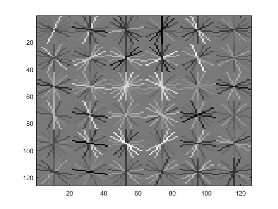
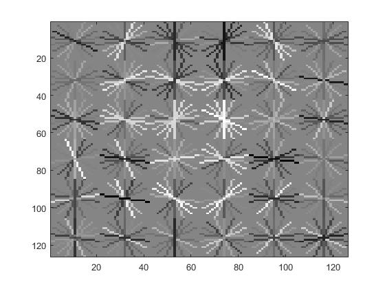
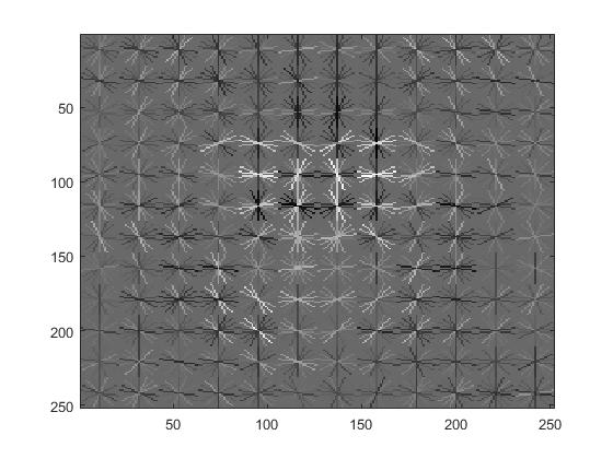
Visualization of this learned classifier.
Precision Recall curve for the developed detector.
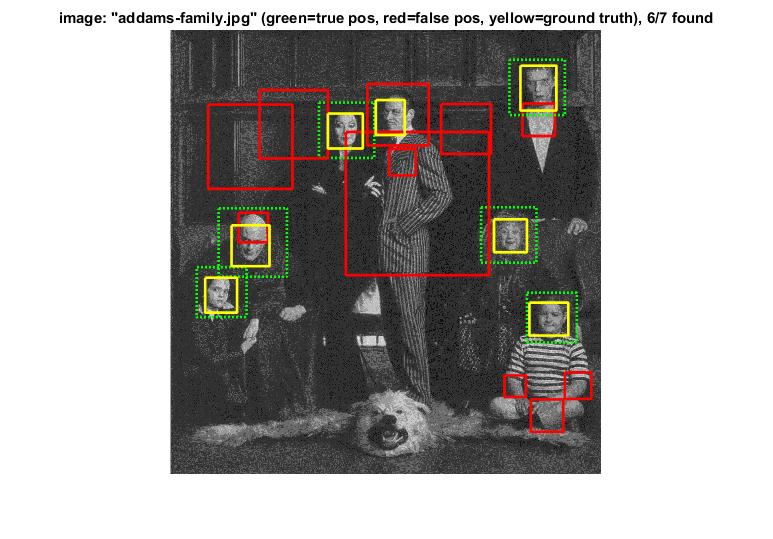
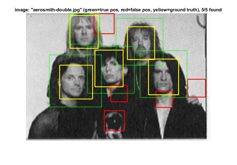
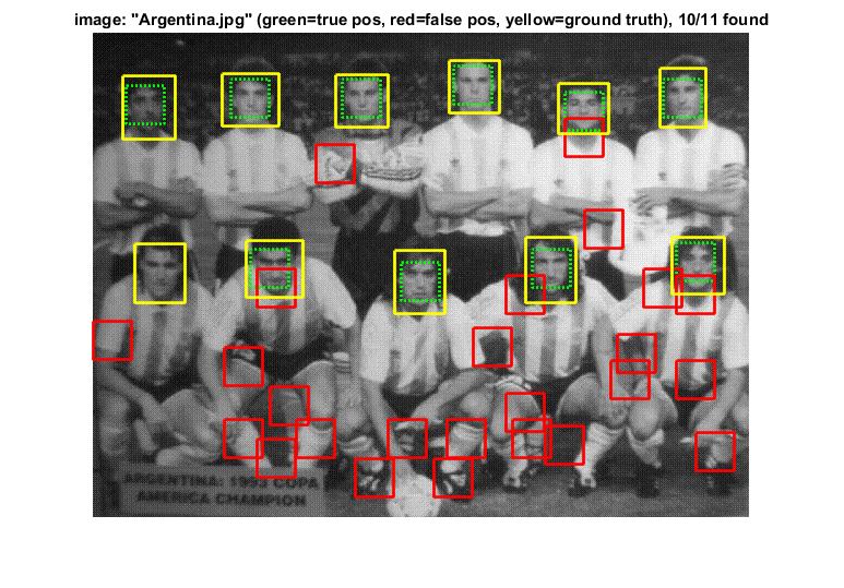
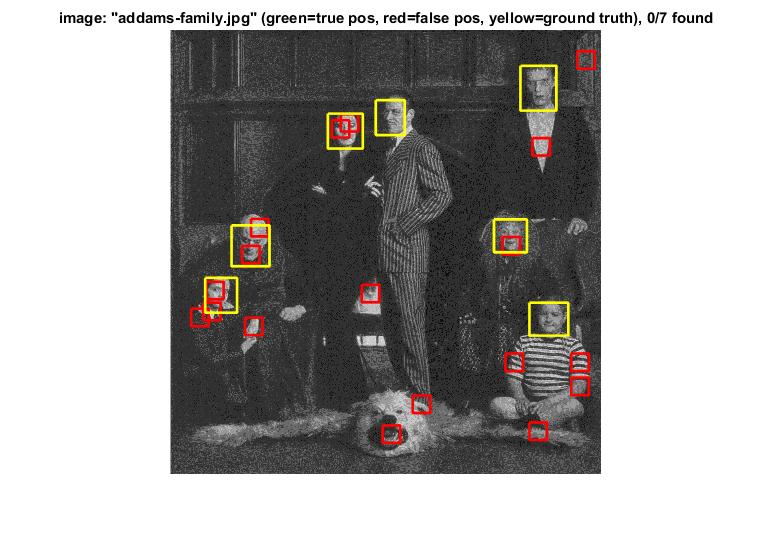
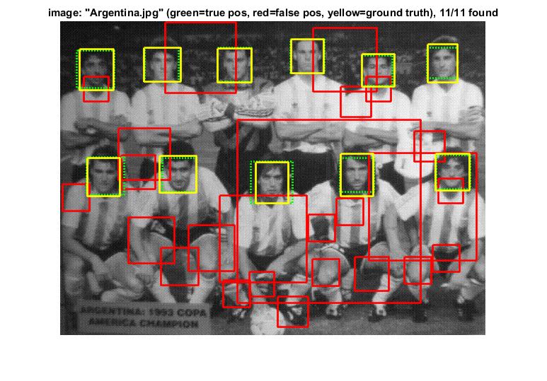
Example of detection on the test set.
Version 2
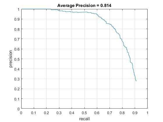
In this version, each test image is downsampled by the scale of 0.7 when the sliding window is applied to detect potential images until the image is smaller than the sliding window. In this case, the average precision is further improved to 0.814. The training time is close to the previous version around 315s. The testing time for all images is around 163s. The visualization of the learned classifier, precision recall curve, and the results of some test images are shown as follows.
Visualization of this learned classifier.
Precision Recall curve for the developed detector.
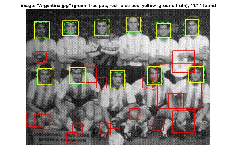
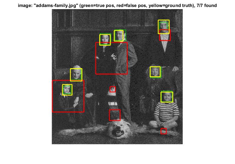
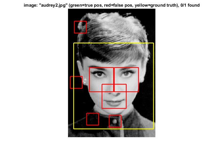
Example of detection on the test set.
Here are some examples of detection faiulure.
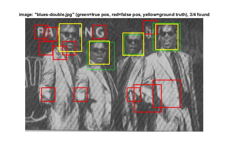
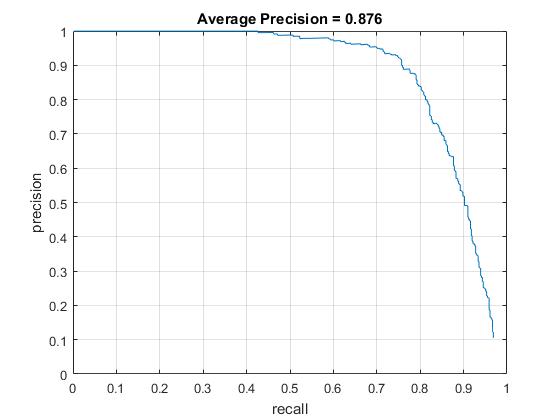
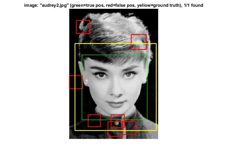
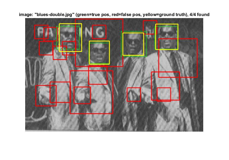
Then, the downsample scale is changed to 0.9, which makes the detection more precise. The average precision is further improved to 0.876. The testing time for all images is around 430s. The visualization of the learned classifier, precision recall curve, and the results of some test images are shown as follows. The two test images which the previous detector fails to detect faces work well with the current face dector.
Precision Recall curve for the developed detector.
Example of detection on the test set.
Version 3
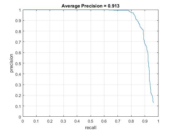
In this version, by keeping all the previous changes, we have changed the HOG cell size, which is also the sliding window step size, to 3. Therefore, more precise detection has been implemented. The average precision is further improved to 0.913. The visualization of the learned classifier, precision recall curve, and the results of some test images are shown as follows.
Visualization of this learned classifier.
Precision Recall curve for the developed detector.
Example of detection on the test set.
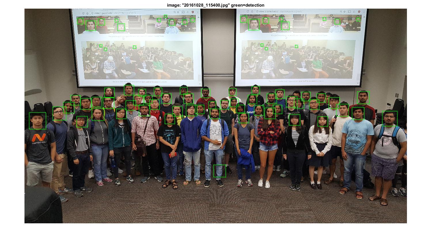
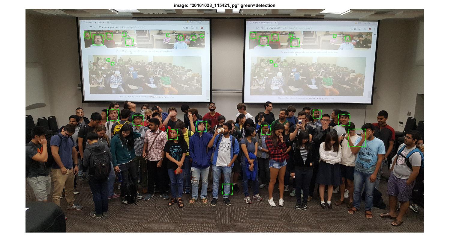
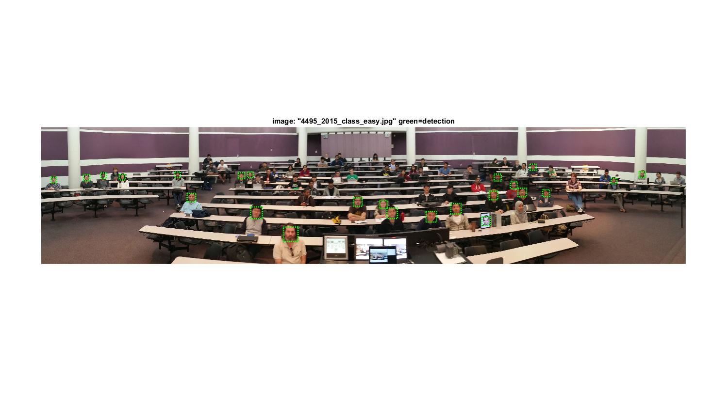
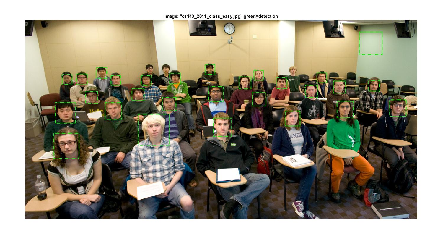
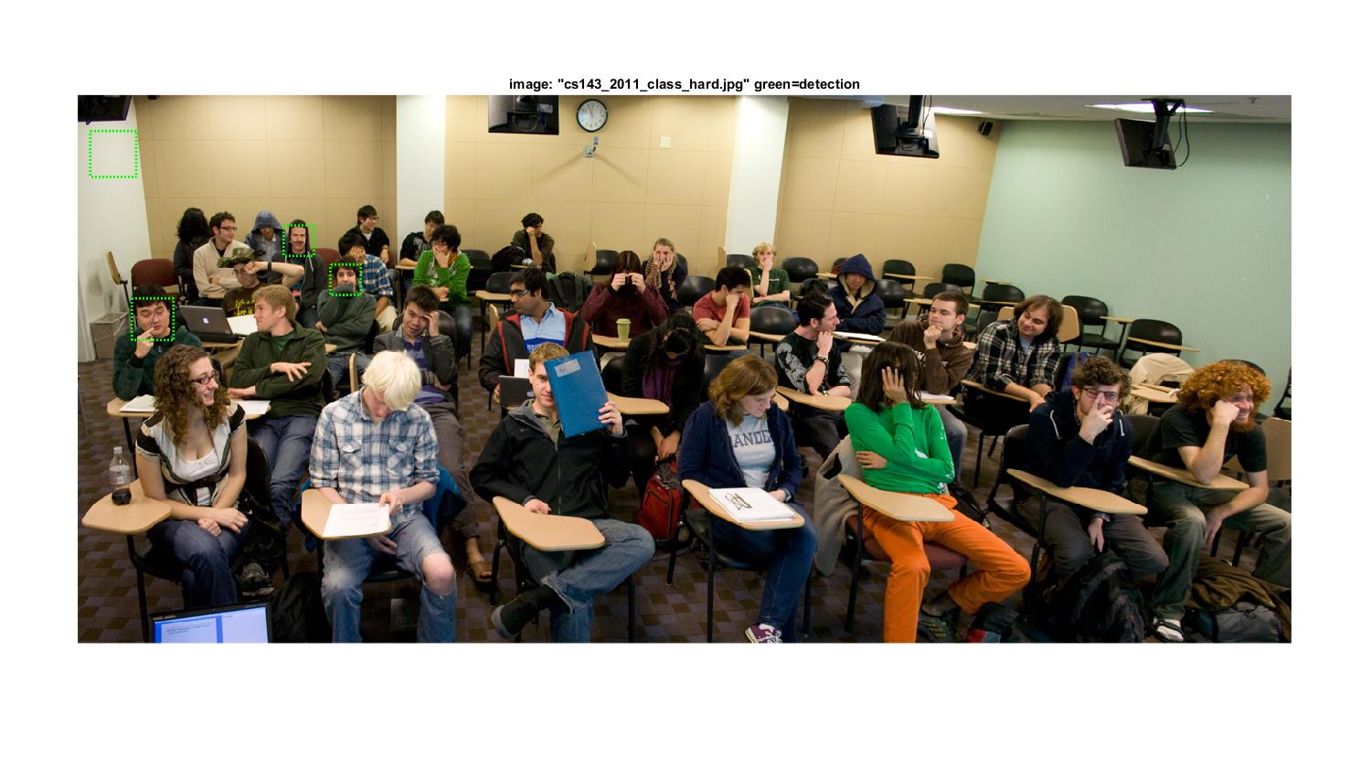
By using this revised version of face detector with HOG cell size equal to 3, extra images taken from classes are tested and the results are shown as follows. In order to eliminate many false positives, the threshold is increased to 1.5 in this case.
Extra Credit
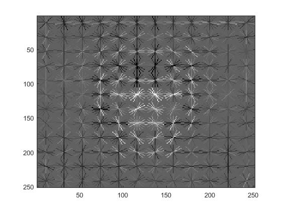
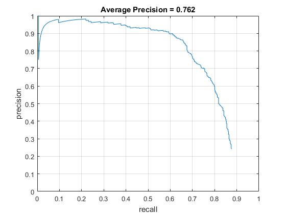
The extra positive training database is taken from LFW database. By setting the HOG cell size as 6 and downsample scale as 0.9, the average precision is 0.762. The visualization of the learned classifier, precision recall curve, and the results of some test images are shown as follows. Compared with the results using the positive database from Caltech Web Faces project, the face regions detected by this detector are usually larger than the ground truth, because the positive examples from LFW database are usually larger than the head regions. Therefore, a simple conclusion is that the quality of positive database is critical to the detection precision.
Visualization of this learned classifier.
Precision Recall curve for the developed detector.
Example of detection on the test set.