Project 5 / Face Detection with a Sliding Window
The goal of this project is to develop a model capable of detecting faces in sets of images. In particular, we will be implementing Dalal and Triggs 2005 sliding window detector. We can distinguish 3 main stages:
- Extract positive and negative features:
At this stage we loaded both positive and negative examples and computed their HoG features. In order to improve perfomance, positive samples were mirrored to increase training data. For negative features we implemented both random negatives extraction and hard negative mining. We will compare perfomances in the Graduate / Extra Credit section.
- Train SVM classifier:
We used a linear classifier, SVM to address this problem. For this purpose we used the inbuilt function
vl_trainsvmfrom the packagevl_feat. - Run classifier on test set:
We used a sliding window to detect faces in different patches of the images. We run multiple experiments with single scale window and multiscale windows, and with different values of HoG cell size.
We will now discuss the results obtained with the different parameters values used at each stage.
1. Single Scale vs Multiscale
We made comparison of performance using single scale window vs multiscale windows:
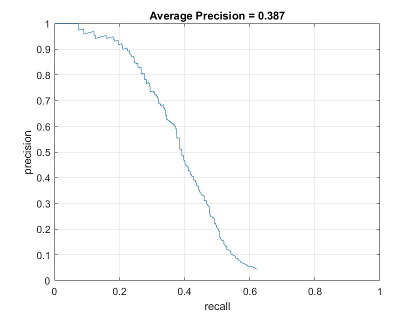
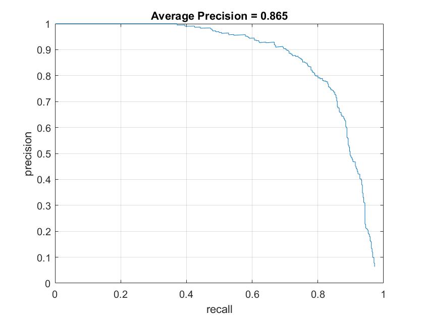
Figure 1. Average precision using one single scale (left) and multiple scales (right).
As we can see AP improved dramatically when multiple scales where considered. This is a completely understandable behaviour, since faces in an image could be of any size.
The values of the rest of the parameters were:
- Number of positive features: 13,426 (sample images + mirrored images)
- Number of negative features: 13,700
- Hard negative mining: no
- Lambda (SVM): 0.0001
- Scale factor: 0.9
- HoG cell size: 6
2. Scale factor in multiscale windows
Next we experimented with different scale factors. The higher the scale factor the more continously windows will be downsampled. We should expect better average precision values but with the downside of higher computation times. This was confirmed by the experiments run:
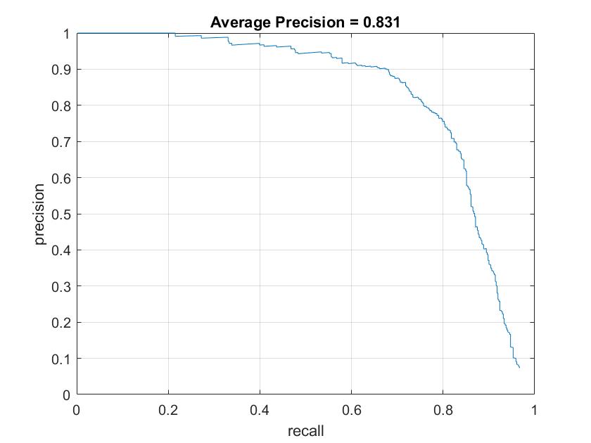
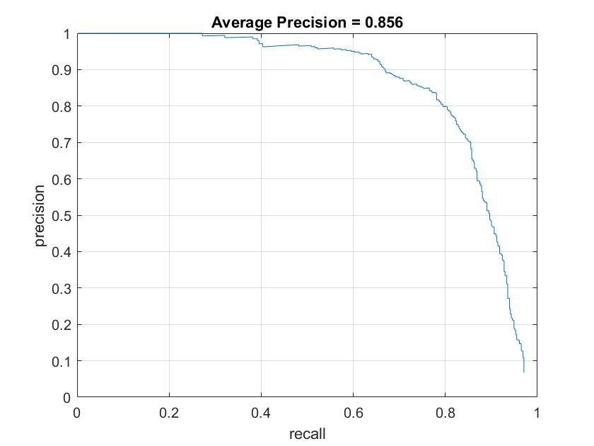
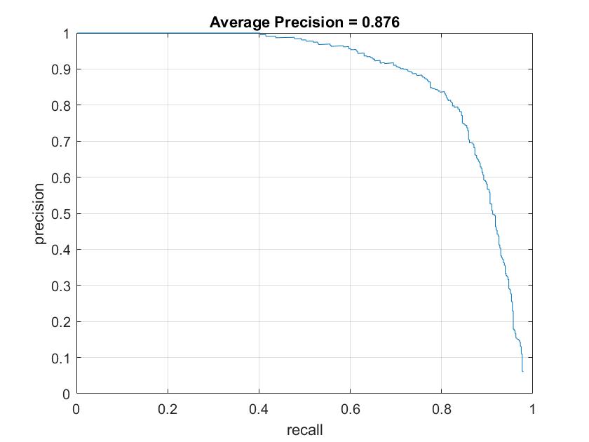
Figure 2. Average precision using multiple scale factors: 0.7(top left), 0.8 (top right), 0.9 (bottom left), and 0.95 (bottom right).

Table 1. Run times using multiple scale factors.
The rest of parameters values were the same as in the previous section.
3. Lambda (SVM)
Next, we experimented using different values of lambda for our SVM classifier. Here are some of the results:

Table 2. AP for different values of lambda.
As we can see, the model's precision is sensitive to lambda values, however, the differences are not too significant for the best results (~0.87). We used scale factor of 0.95. The rest of the parameters values were the same as previously.
4. HoG cell size
At this point, we decided to experiment changing HoG cell size value, that is, we experimented with the number of HoG features extracted from each patch of the image. The lower the HoG cell size, the more HoG features will be extracted. Here are the results obtained:

Table 3. AP for different values of HoG cell size.
It must be noticed that as HoG cell size decreases, run time increases exponentially. Lambda = 0.0001, scale factor = 0.95
5. Hard Negative Mining (Graduate / Extra Credit)
As graduate credit, we decided to implement hard negative mining. For this experiment, we reduced the number of initial negative samples to 5000. As we can see, when the number of negative samples is limited, hard negative mining can significantly improve precision. In concrete, the results obtained were as follows:

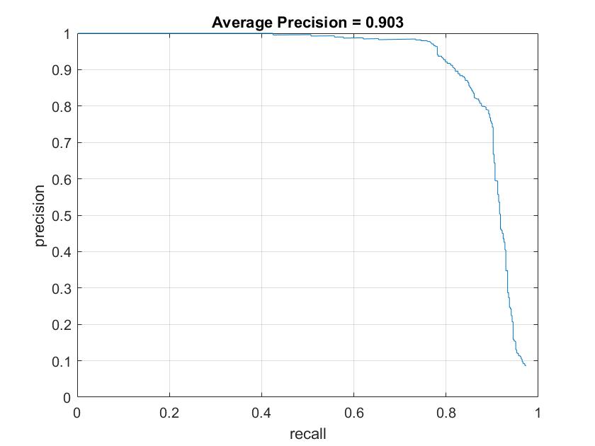
Figure 3. AP with random negative samples (left) and hard negative mining (right).
6. Best model
After trying multiple experiments, our best model was reached with the following parameter values. Surprinsingly our best model was obtained in one of our first implementations, here are the details:
- Number of positive features: 6,713 (original sample images)
- Number of negative features: 13,700
- Hard negative mining: no
- Lambda (SVM): 0.0001
- Scale factor: 0.95
- HoG cell size: 4
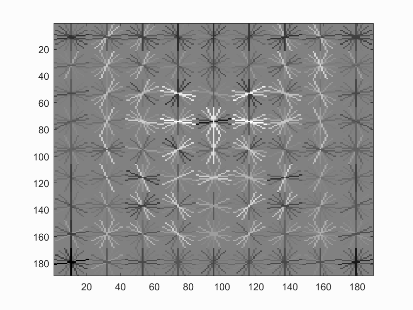
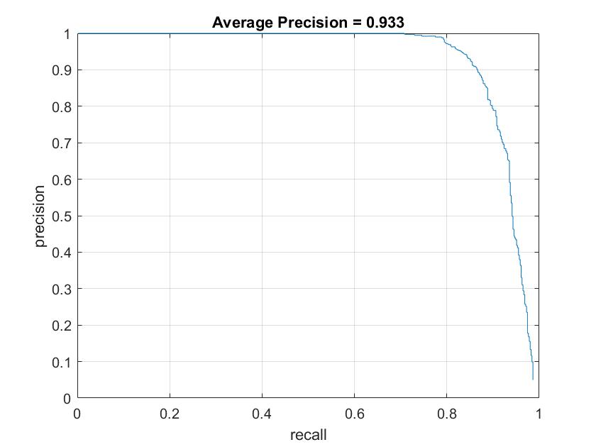
Here are some visualizations obtained with our best model:
Face template HoG visualization.
Precision Recall curve.
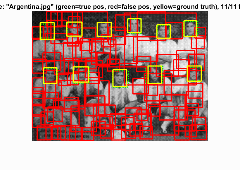
Example of detection on the test set.
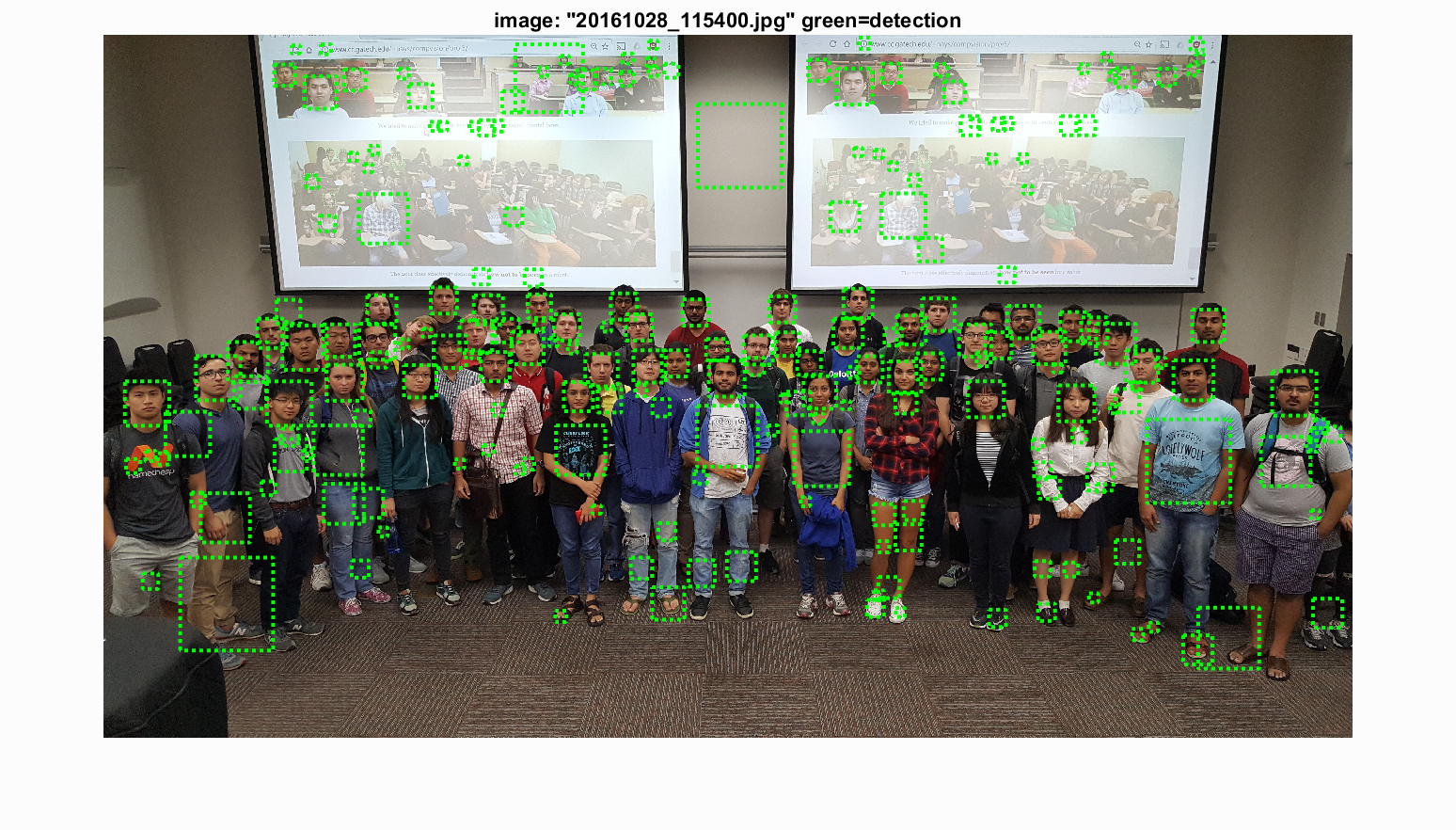
Class images
Class image 1.
Class image 2.
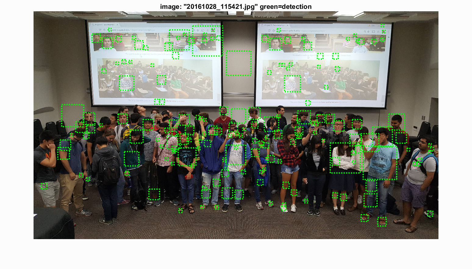
Due to time constraints, we reduced the scale factor to 0.9