Project 5: Face Detection with a Sliding Window

Machine Learning was used to train an algorithm to detect faces in images via a sliding window. A Support Vector Machine (SVM) was trained with different positive and negative data, and used to test data in a different image sample. The algorithm had high accuracy on out of sample data, and detected most of the faces in the images tested.

The basic pipeline of this approach follows the steps below:

1. Get Histogram of Oriented Gradients (HOG) descriptor for negative and positive face examples.
2. Train linear SVM.
3. Slide window at multiple scales and detect potential face like.
4. Non-maxima suppression on the results in each image.

In addition, the following items have been implemented for extra credits:

1. Hard Negative Mining (up to 10 pts)
2. Finding and utilizing alternative positive training data (up to 10 pts)

Positive and Negative Training Data

Positive training example: 6,713 cropped of 36x36 faces image from the Caltech Web Faces project.

Negative training example: 10,000 non face, randomly chosen from Wu et al. and the SUN scene database.

Training an SVM

Now that we have positive and negative samples, we will train an SVM to classify faces from non-faces. Then, we crop out sections of the test images to see if we can classify faces. This is done in the following manner:

1. Scale image by a scaling factor (Geometric progression of 0.9).
2. Implement HOG on the scaled image.
3. Slide a window over the HOGed image. (the window size should match that of the trained examples).
4. Multiply the test window by the weights and biases learned by the SVM and get a confidence score.
5. If confidence is above a certain value, then cut a scaled bounding box of the size of the window and save this box.
6. Perform Non-maximum suppression over all the boxes to get a better estimated of detected faces.

Designing Parameters

Determining Detection Threshold

The evaluation function used in this project does not seem to include false positives in its calculation of Average Precision, so it is difficult to judge the threshold without visually looking at the results. After trying different values, I settled on 0.4, because it had the best overall results.

Effect of the parameter, Lambda, with fixed other parameters: HOG cell size(6), Detection Threshold(0.4).

Lambda	0.001	0.0001	0.00001
AP (%)	75.3	86.7	81.7

HOG features with different cell sizes

The size of the HOG cell used for the images was very important. A smaller HOG cell means that more features are likely to be detected because the window over which the image is processed is smaller. However, smaller HOG cell size also meant longer running time. I tried HOG cell sizes of 3, 4, and 6 to verify its quantative effectiveness on the average precision.

Other fixed parameters: Lambda for SVM(0.0001) and Detection Threshold(0.4).

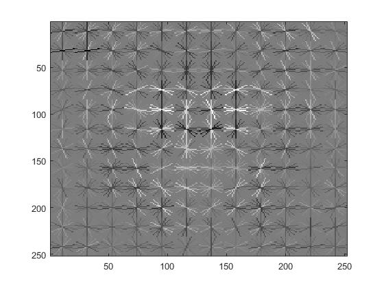
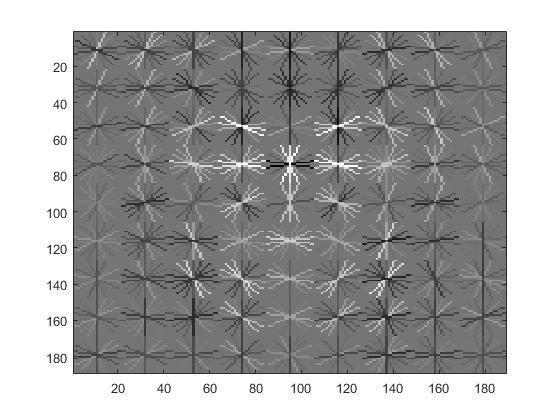
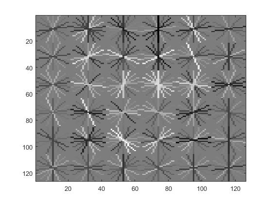
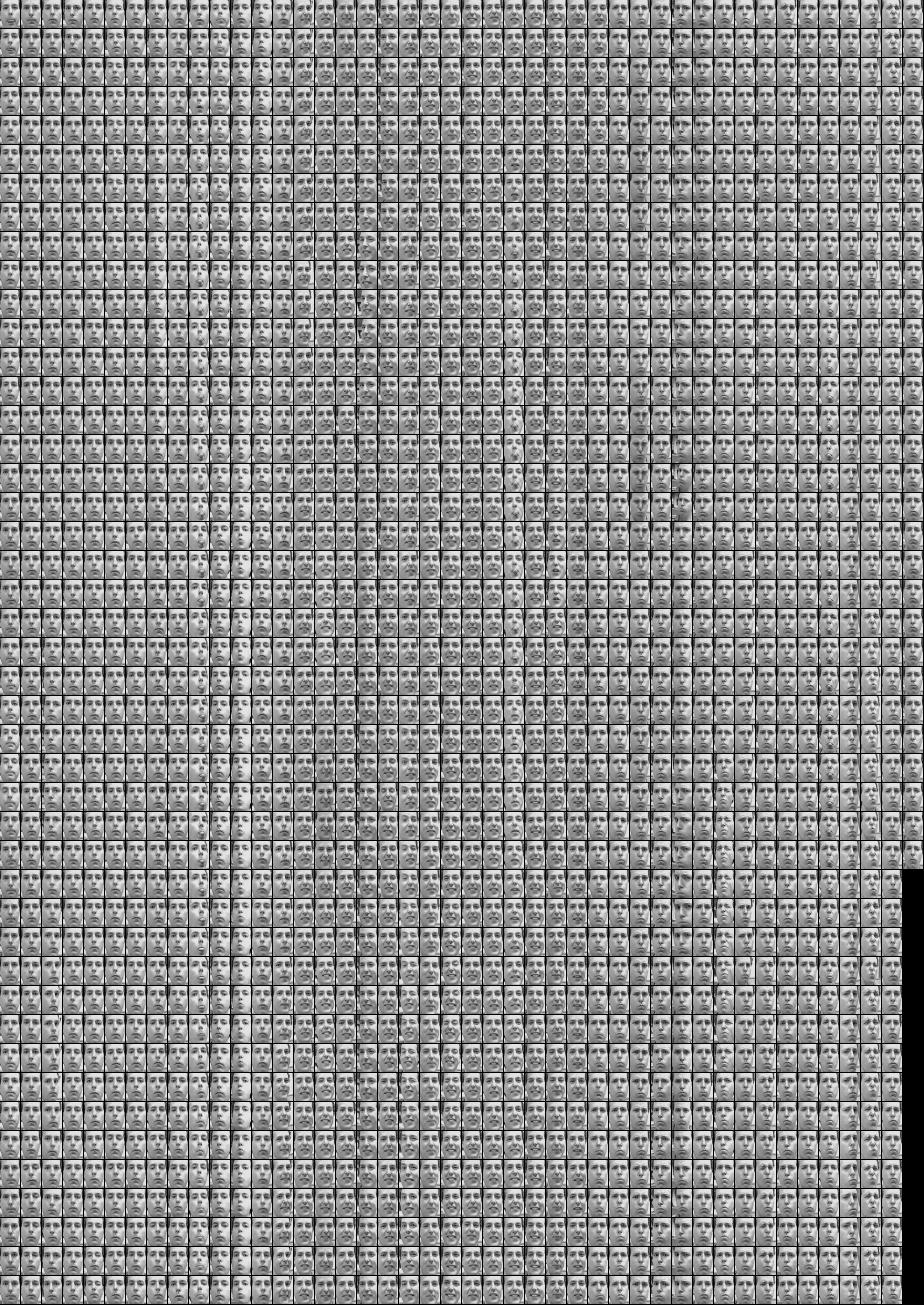
Visualization of HOG features with cell sizes of 3, 4, and 6, respectively.

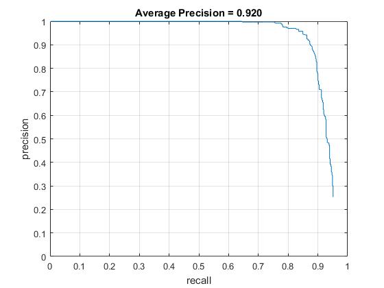
Average precision with HOG cell sizes of 3, 4, and 6, respectively.

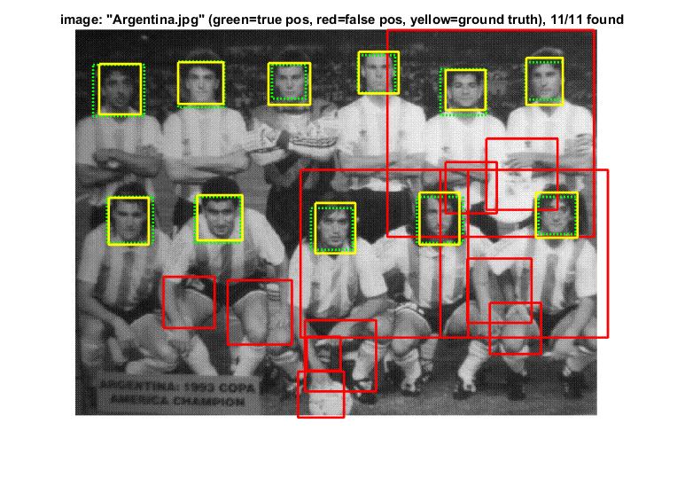
Face detections on "Argentina.jpg" with HOG cell sizes of 3, 4, and 6, respectively.

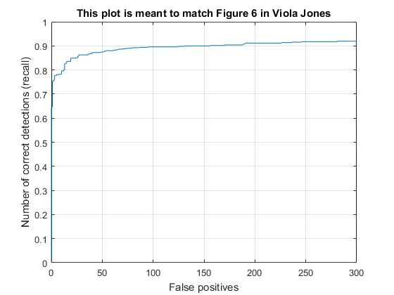
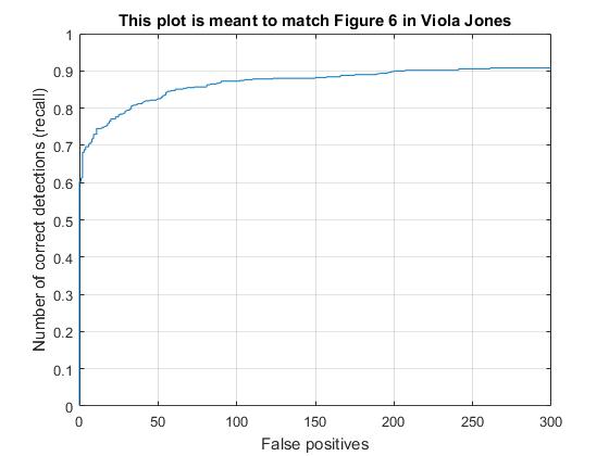
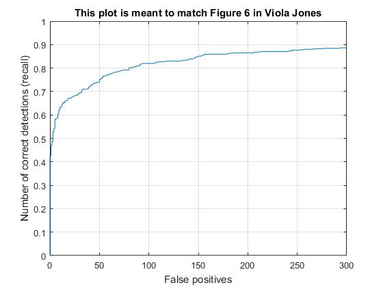
Recall vs False positive plot with HOG cell sizes of 3, 4, and 6, respectively.

With the HOG+SVM architecture and a HOG cell size of 3, I achieved the average accuracy of 92% However, it took much longer time (~10 min.) to run the code while the code with HOG cell size 6 took less than 2 minutes. Moreover, HOG cell size does not significantly improve to reduce false positive as shown in the result of face detection and the recall vs false positive plot. This is the reason why hard negative minining is necessarily implemented which will be discussed in the follwing extra credit section.

Extra Credits

1. Hard Negative Mining (up to 10 pts)

To reduce false positives, Hard Negative Mining can be chalked out as follows:

1. Train the SVM from the positives and 10,000 random negatives (as described in previous sections).
2. Now, use the part of the training set without any faces to test our SVM (instead of the testing set).
3. Append all the detected faces (false positives) to the training set as negative examples.
4. Retrain the SVM using this appended dataset and test on the test set.

The code for the above described algorithm should be placed on the 'step 4. (optional extra credit) Mine hard negatives' section with the function 'hard_neg_mining.m':

features_false_pos = hard_neg_mining(non_face_scn_path, w, b, feature_params);
features_all = [features_all; features_false_pos];
labels = [labels; (-1)*ones(size(features_false_pos, 1), 1)];
[w b] = vl_svmtrain(features_all', labels, LAMBDA);

Since all the positives detected by the original 'run_detector.m' function are false positives, the 'hard_neg_mining.m' function is very similar to the previous one. There are only two modifications: 1) The function returns cropped false positive HOG features instead of true positives and 2) There is no non-maximum suppression since we don't need it.

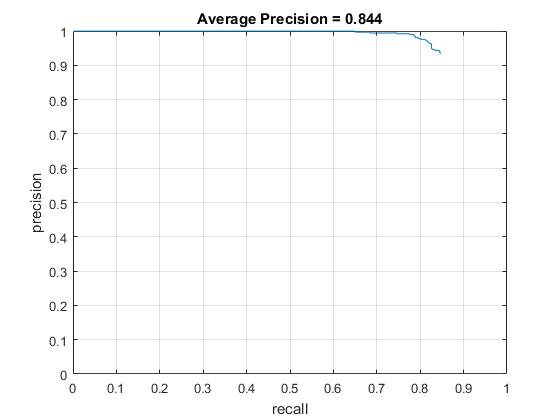
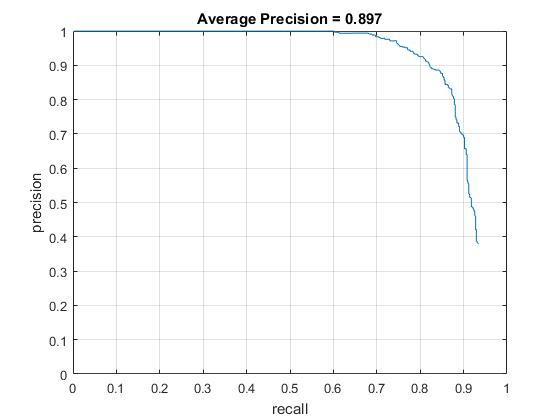
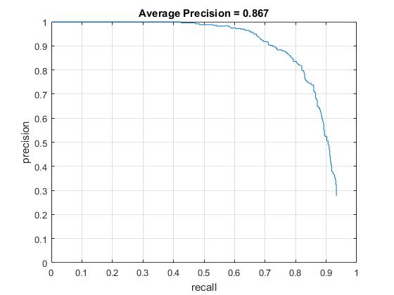
Average Prevision after/before Hard Negative Mining with HOG cell sizes of 3.

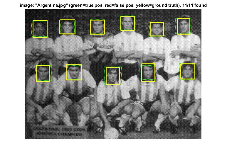
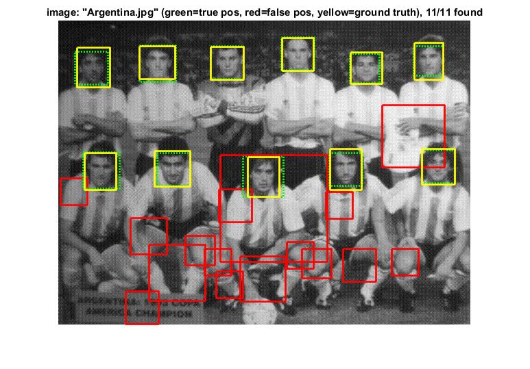
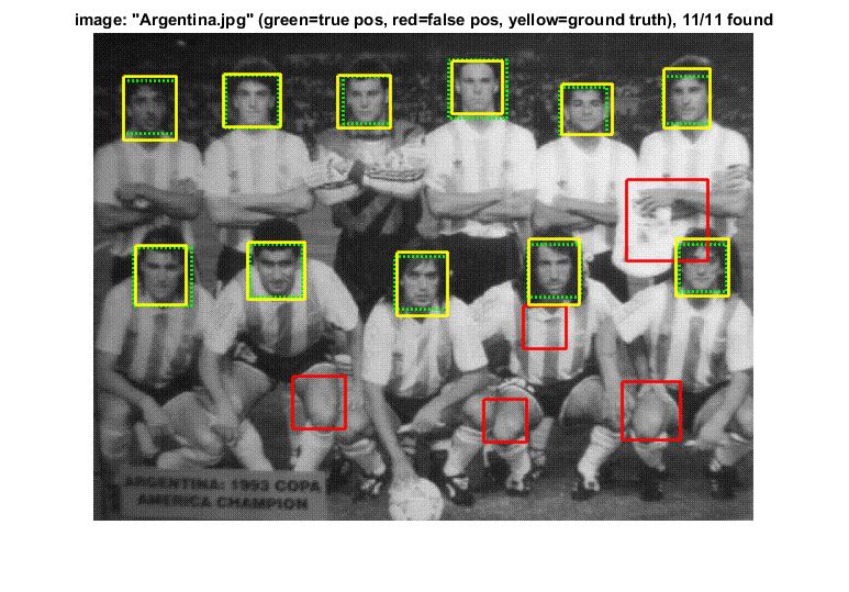
"Argentina.jpg" after/before Hard Negative Mining with HOG cell sizes of 3.

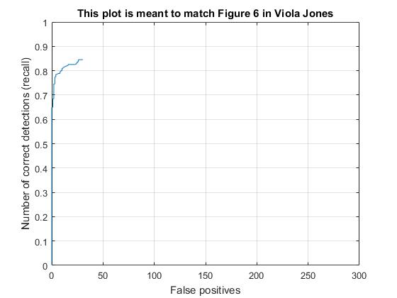
Recall vs False positives plot after/before Hard Negative Mining with HOG cell sizes of 3.

Though the average precision after Hard Negative Mining droped from 92.0% to 84.4%, it showed sigificant improvement on reducing false positives.

2. Finding and utilizing alternative positive training data (up to 10 pts)

I looked for extra training data sets for faces, and found several image sets which are Frey Faces(20x28 size, 1,965 images), Olivetti Faces(64x64 size, 400 images), and UMist Faces (112x92 size, 575 images). I used the data available on the following page: http://www.cs.nyu.edu/~roweis/data.html. Total 2,940 extra face images were resized to 36x36 and used in 2 cases: 1) replaced positive training set and 2) additional positive training set.

Frey Faces(20x28 size, 1,965 images)

Olivetti Faces(64x64 size, 400 images)

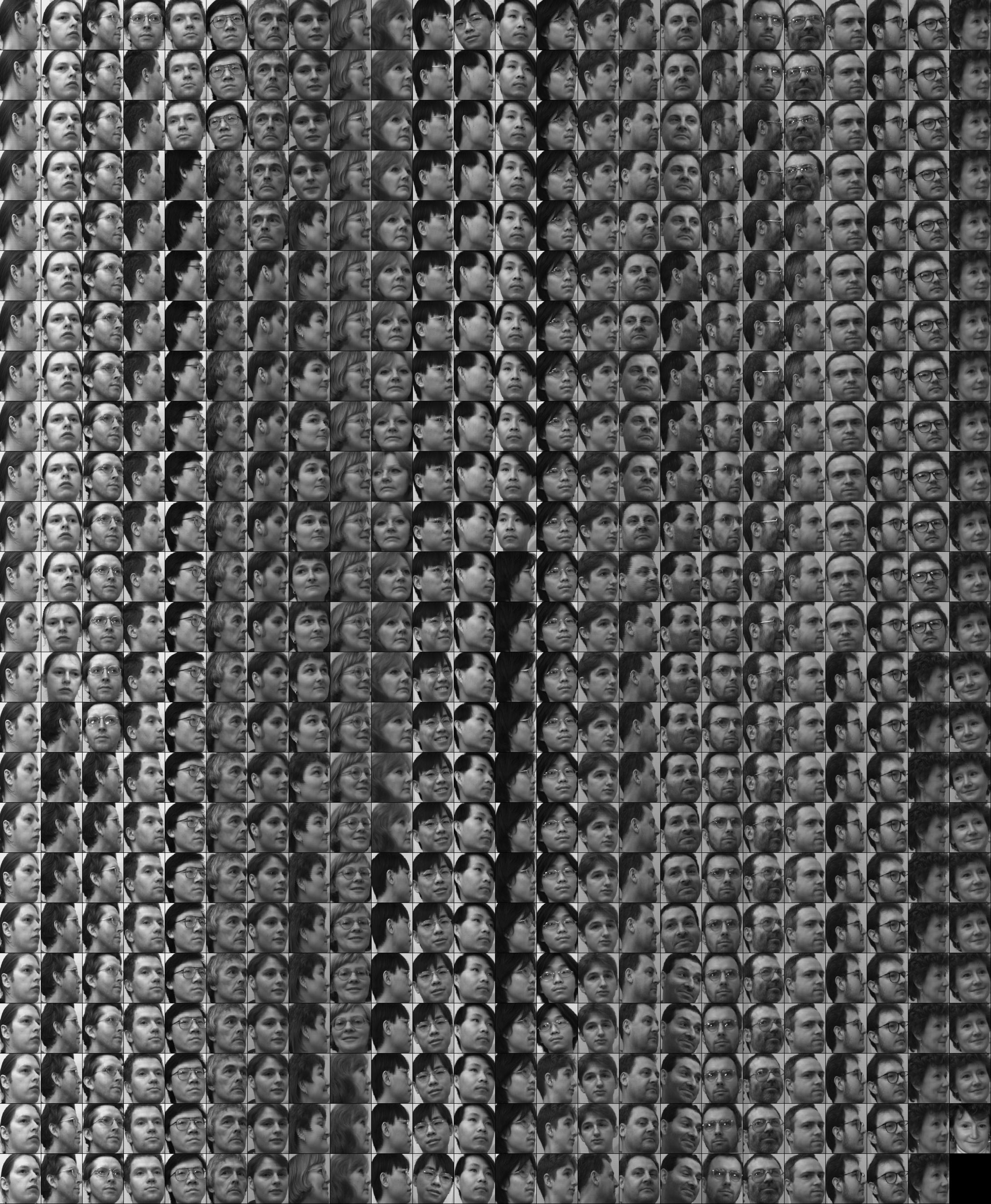
UMist Faces (112x92 size, 575 images)

When the new face images only were used for positive training data, the average precision was dropped drastically from 80~90% to 50~60%. This makes sense since I used less than half number of training data. However, the average precision did not become significantly better when I added the extra face images to the original positive training data (86.7% -> 88.4%, increased by 1.7% with HOG size of 6 and 92.0% -> 89.6%, decreased by 2.4% with HOG size of 3). Though the more positive training data work better, generally, I think this is because of the quaility of the extra face images. The extra set contains a lot of side faces which possibly makes a confusion with the other positive training data.

Result of Extra Positive Traning Data

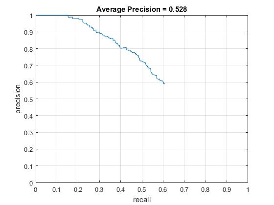
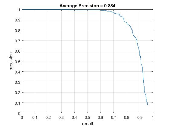
Average Prevision of replaced/additional positive training set with HOG cell sizes of 6.

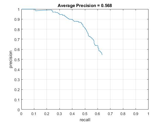
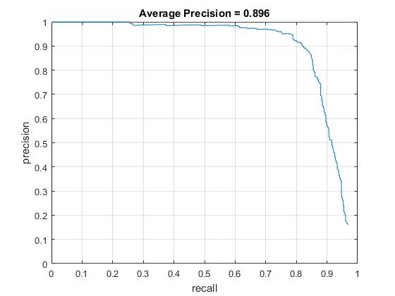
Average Prevision of replaced/additional positive training set with HOG cell sizes of 3.

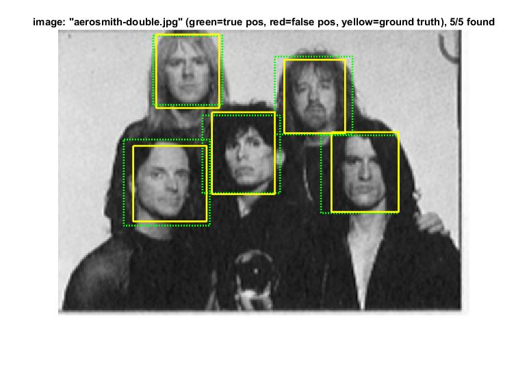
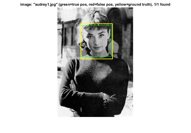
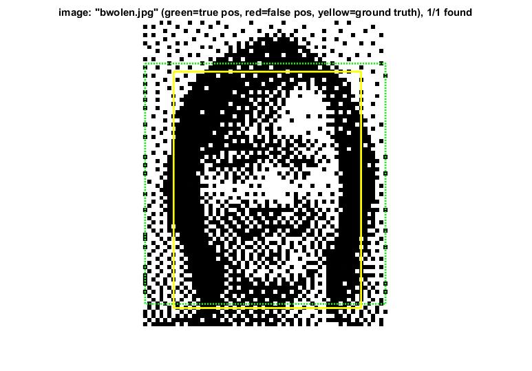
Visualization of Face Detection Results (HOG cell size 3 + Hard Negative Mining)
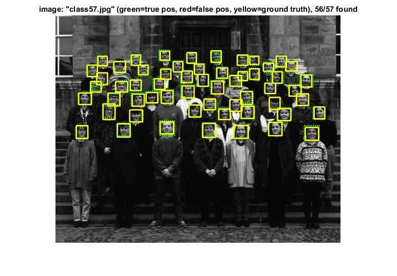
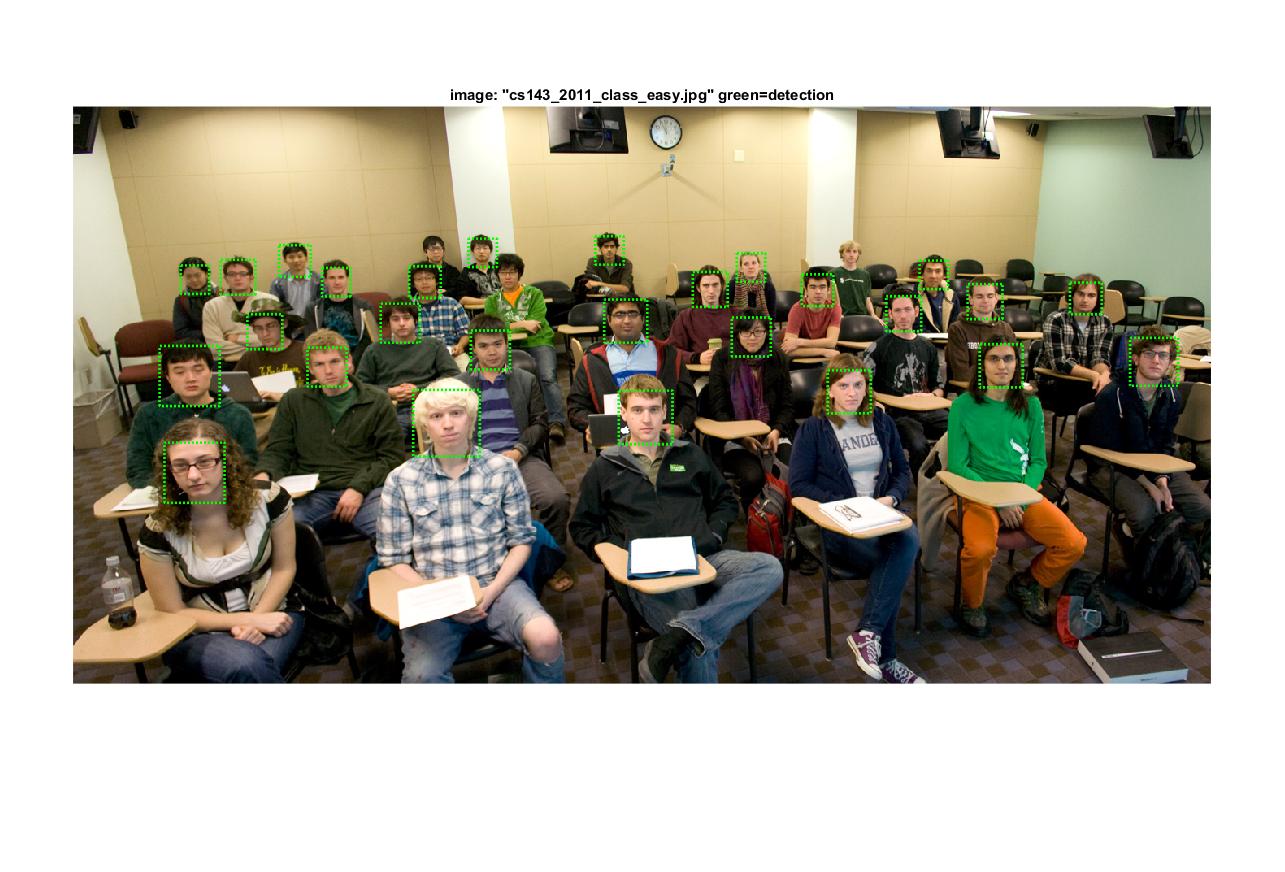
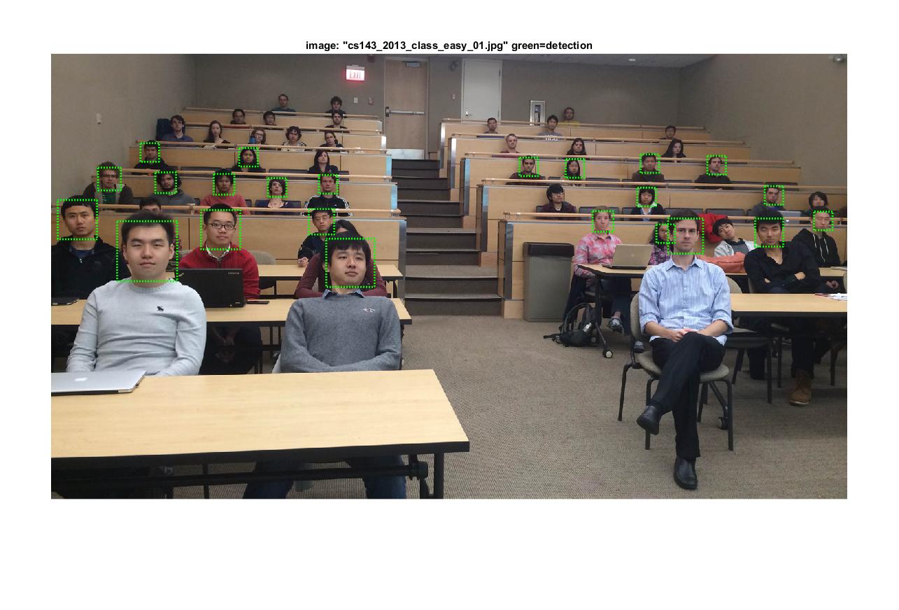
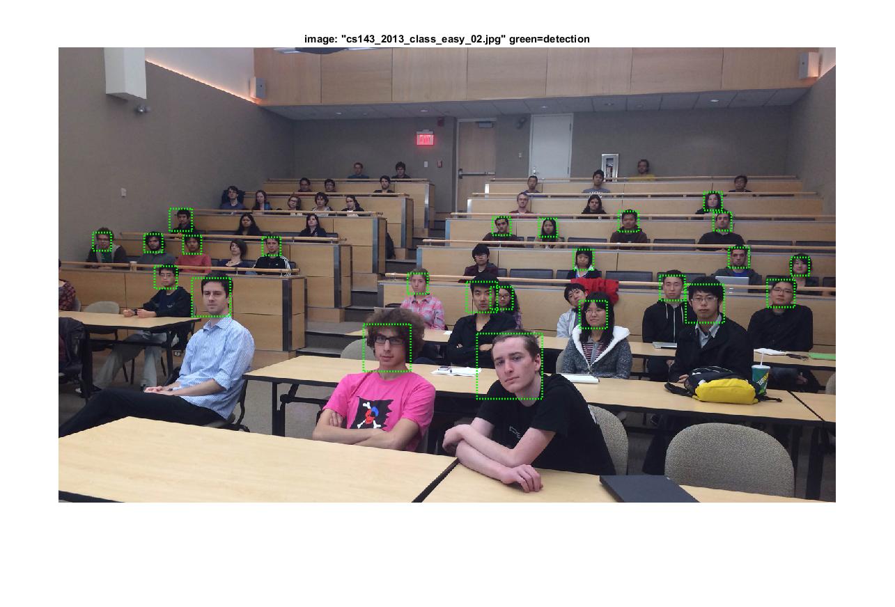
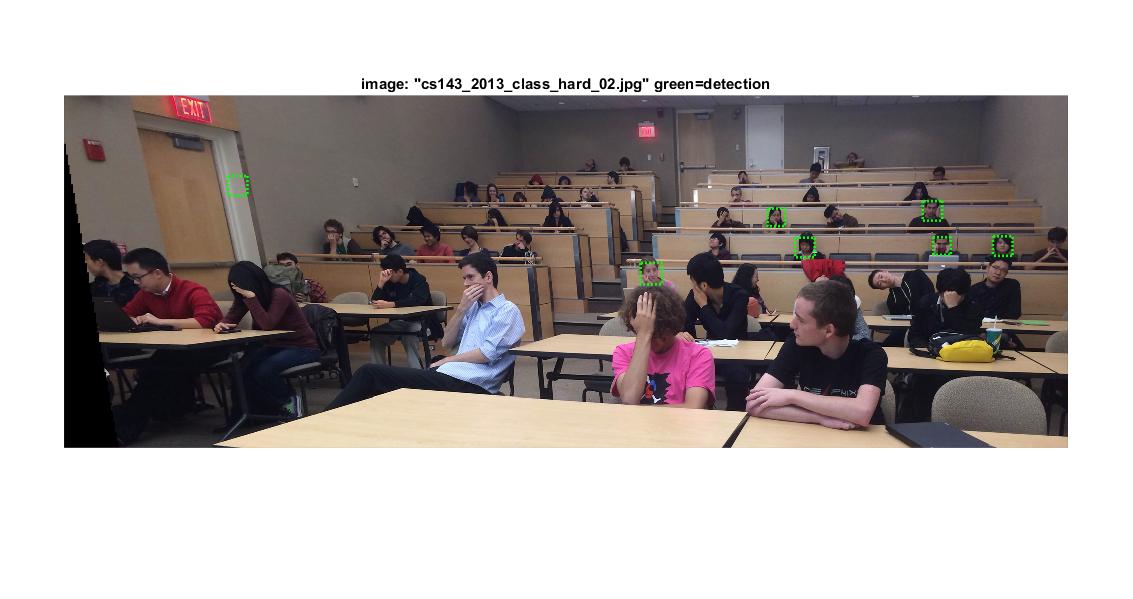
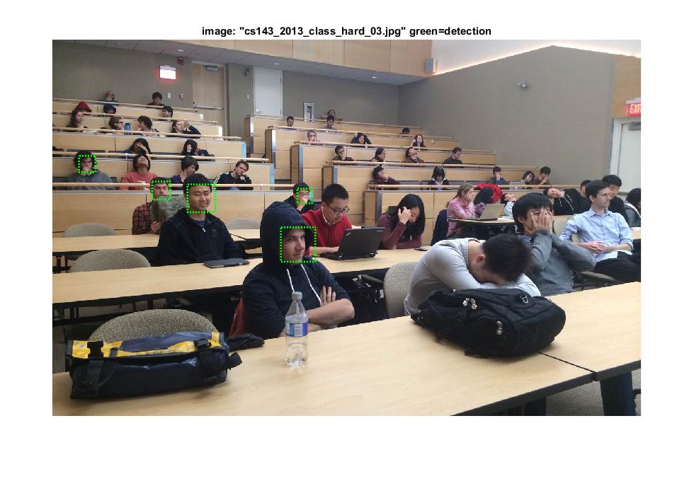