Project 5 / Face Detection with a Sliding Window
In this project, I implemented the sliding window detector as written in a paper by Dalal and Triggs. There were four functions we had to implement for this project:
- Getting Positive Features
- Getting Random Negative Features
- Classifier Training
- Running the Detector
Getting Positive Features
I get each image and compute the Histogram of Oriented Gradients using vl_hog.
Getting Random Negative Features
For a random image, I grayscaled it. Then I get random samples of the image and use vl_hog to find the HOG and add it on to the negative training examples.
Classifier Training
I call vl_svmtrain for the classifier training from the data vectors, positive and negative features, and the labels, 1's and -1's, and the lambda as .0001.
Running the Detector
I basically convert each image to HOG feature space using vl_hog for each scale. I take the Hog spaces and create a space with them. I then use a confidence level of .75 to find greater than that.
Example Code: classifier_training
function [w, b] = classifier_training(features_pos, features_neg)

	features_pos = features_pos';
	[~, numbers_pos] = size(features_pos);

	features_neg = features_neg';
	[~, numbers_neg] = size(features_neg);

	labels = ones(1, (numbers_pos + numbers_neg));
	labels(numbers_pos + 1 : end) = -1 * labels(numbers_pos + 1 : end);

	[w, b] = vl_svmtrain([features_pos, features_neg], labels, 0.0001);

end
Results in a table
|
|
|
|
|
|
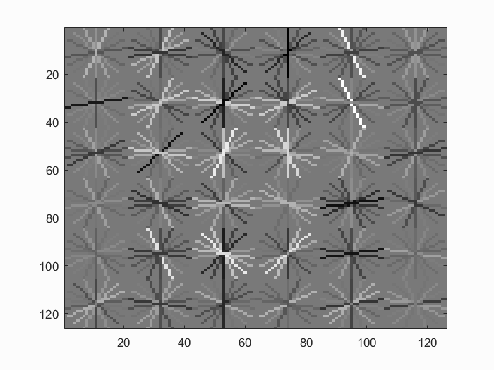
Face template HoG visualization learned after training data. It looks roughly like a face after classifier training.
Precision Recall curve for the test data.
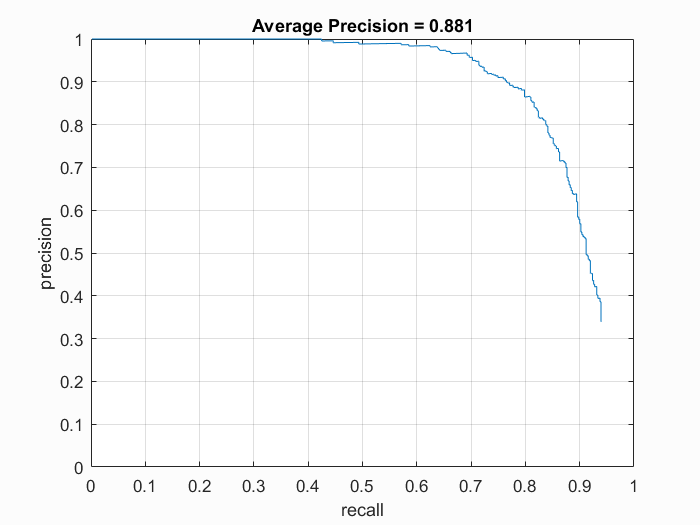
Average precision came to be .881. As can be seen, the sliding window detector worked pretty well.
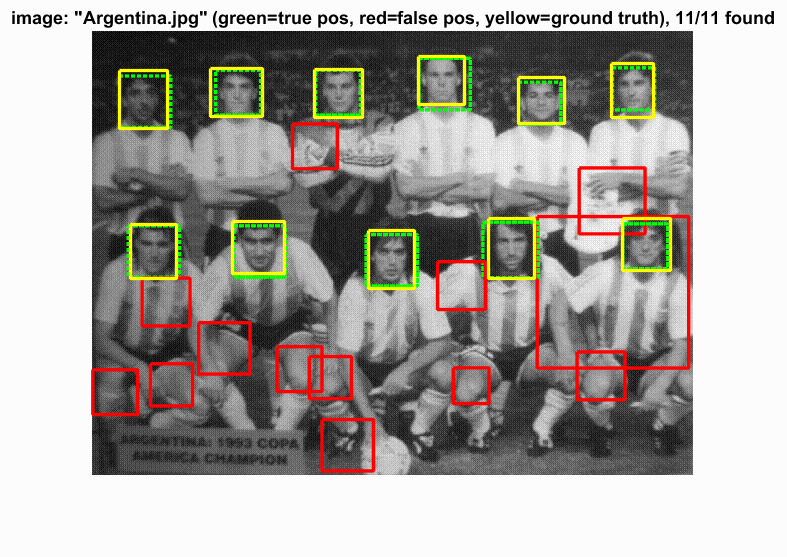
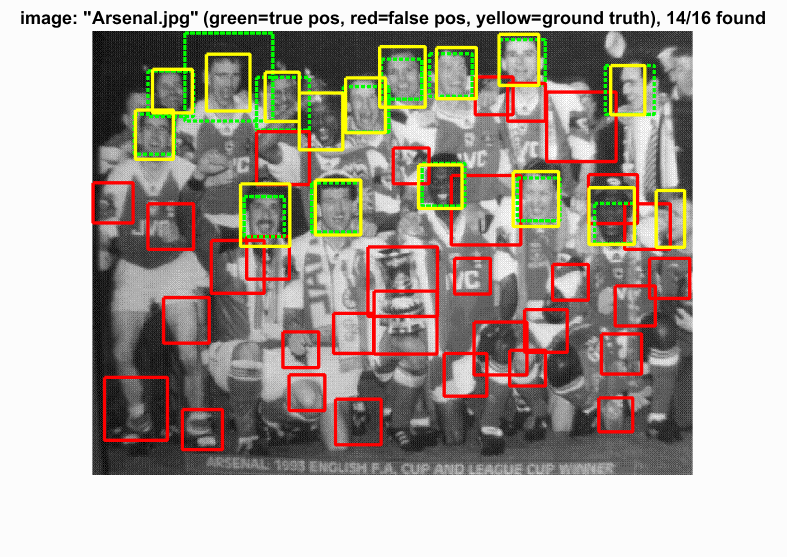
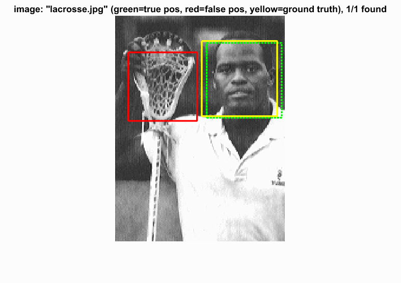
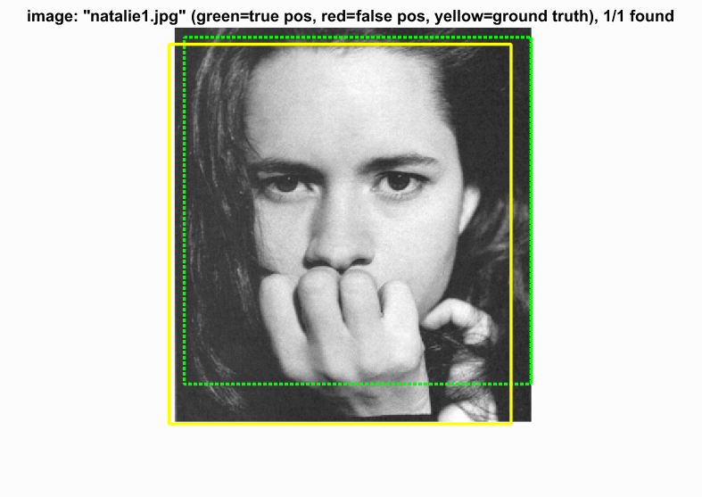
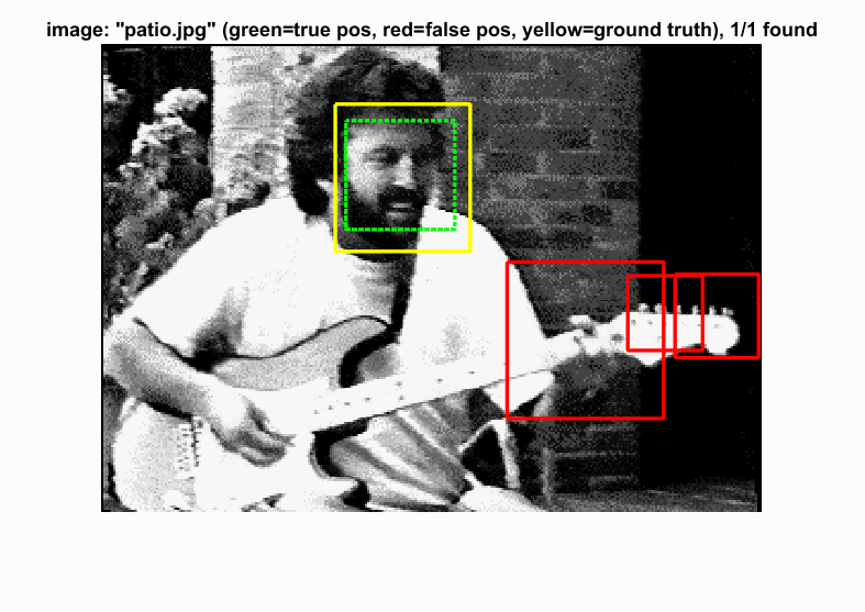
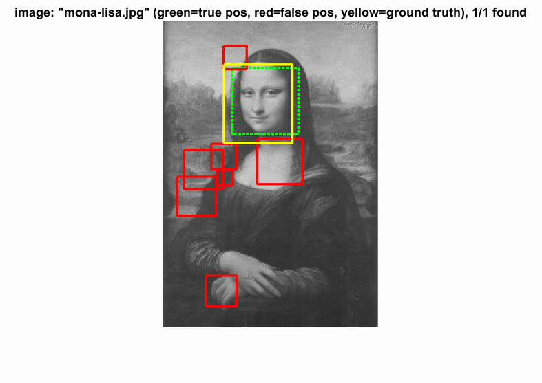
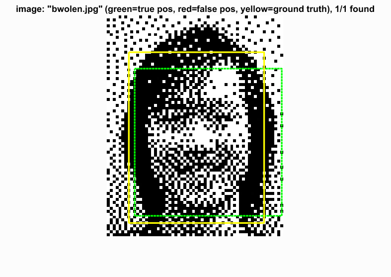
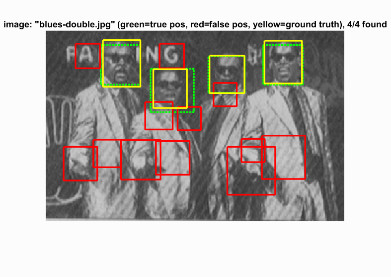
Test Scenes
Initial classifier performance on train data:
- accuracy: 0.998
- true positive rate: 0.400
- false positive rate: 0.000
- true negative rate: 0.598
- false negative rate: 0.001
vl_hog: descriptor: [6 x 6 x 31]
vl_hog: glyph image: [126 x 126]
vl_hog: number of orientations: 9
vl_hog: variant: UOCTTI