Computer Vision Project

Project 5: Face Detection with a Sliding Window

Author: Mitchell Manguno (mmanguno3)

Table of Contents
Synopsis
Pt. 1: Training Data
Pt. 2: SVM Training
Pt. 3: Detection
Results

Synopsis

For this project, a basic facial detection pipeline was implemented. First training data was culled from both positive examples and negative examples. In the case of negative examples, singular images were sampled many times for many negative samples (to boost training). These samples (in both cases) were transformed into HoG vectors to more accurately describe eachs sample. Second, a linear SVM was trained on this data, resulting in a tuple of W and b. Finally, candidate images were tested for the existance and location of faces with a sliding window, both with single and multi-scaling.

We begin the discussion with part 1, training data culling.

Pt. 1: Training Data

As we are using a linear SVM to discern the confidence of elements within our sliding window, we require training data. Our positive examples are easy: we have 36x36 cropped images of faces provided. All we had to do is extract a HoG vector from it:


% Iterate over all images, resize, calculate HoG features, and resize
for i=1:num_images
    image = I[i]
    hog_vector = hog(img, hog_cell_size);
    H[i] = hog_vector
end
return H

There is one free variable here, hog_cell_size, which refers to the size (in pixels) of each cell in the HoG vector. It was set to 3 for time constraints (the lower the cell size, the higher the granularity, and the longer it takes).

For the negative features, it was a bit different: all that has to be done is randomly choose some 36x36 cropping of the image, and let that be the negative feature. Since any 36x36 patch of the image is negative, we can crop any patch and use it. So, we can crop one image as many times as we want. We do this for more negative samples.


% The number of features, on average, to extract from each image.
num_features = ceil(num_samples / num_images);

% Iterate over all images, resize, calculate HoG features, & resize
for i=1:num_images
    cur_image = I[i]
    for j=1:num_features
        % Get random numbers on interval (1, bound_[x|y]).
        random_x = random(1, bounds(cur_image, 'x'));
        random_y = random(1, bounds(cur_image, 'x'));

        image_patch = cur_image(random_x:random_x+36, random_y:random_y+36);
        hog_vector = hog(image_patch, hog_cell_size);
        H_i[j] = hog_vector
    end
    H[i] = H_i
end

Again, hog_cell_size was 6. We also had a num_samples, which was always at least 10,000 samples.

Pt. 2: SVM Training

For the second part, we trained an SVM based on those samples. This was a fairly simple step.


all_features = concatenate(positive features, negative features)
labels(positive features) = 1
labels(negative features) = -1
[W, b] = SVM(all_features, labels, λ=.001);

As you'd expect, we get a W vector and a b constant with which to evaluate the HoG vectors for a confidence score.

Pt. 3: Detection

In the last part of the pipeline, we do the real work: detecting. Here, we turn the entire image into a HoG vector of size (image_x_size / hog_cell_size)x(image_y_size / hog_cell_size)x31.


hog_vector = hog(img, hog_cell_size);

Then we iterate over this HoG vector, cropping out patches of size (36/hog_cell_size)x(36/hog_cell_size). This patch roughly represents the 36x36 patches of faces we took earlier as training samples, dividing by the cell size since each HoG cell represents that many pixels. For examples, with a hog_cell_size of 6, each HoG patch would be 6x6x31, which corresponds to the 6x6x31 of the training samples. More importantly, this matches up with the W vector of the SVM, for confidence scoring.


for j=1:bound(hog_vector, 'x')-(template_size/hog_cell_size)
    for k=1:bound(hog_vector, 'y')-(template_size/hog_cell_size)

        coords = (y_min, x_min, y_max, x_max) = (k,j,
                                                 j+template_size/hog_cell_size,
                                                 k+template_size/hog_cell_size)

        cur_hog_patch = hog_vector(x_min:x_max, ...
                                   y_min:y_max, :);

        confidence = resize_vector * w + b;
        if confidence > threshold
            Confidences[i] = confidence;
        end
    end
end

Additionally, we take those cropped region and upscale it back to the image's dimensions to get a 'bounding box' around a feature if we detect that it is a face.


Bounding Boxes[i] = coords .* hog_cell_size

Finally, there is a choice of scaling. We can either run such a detection function once over the image, and that would be fine. However, we can also run the detector over the image at ever decreasing scalings of the image, gathering bounding boxes from each.


original_image = img;
for y=0:number_of_scales
    scaling = scale_factor^(y);
    scaled_img = scale(original_image, scaling);
    hog_vector = vl_hog(scaled_img, hog_cell_size);

    % Rest of detection code....
end

In this case, we'd also need to scale up the bounding box corners some more:


Bounding Boxes[i] = coords .* (hog_cell_size/scaling)

In this algorithm, there are 5 parameters to tune:

the size of the hog cells,
the number of negative samples to mine,
the number of times to scale the image,
the scaling factor, and
the confidence threshold.

After many, many painstaking hours of parameter tuning, I came across the best settings for these parameters that I could find. I chose to scale the image 2 times with a scale factor of .6, and to threshold the images lower than a confidence of -3. For the HoG cells, a size of 6 I found to be best, given the time constraint. Changes to these parameters did not make any substantive increase to accuracy (and if they did, the increase in time was not worth the few percentage points).

Results

Single-scale


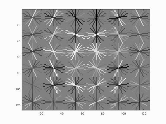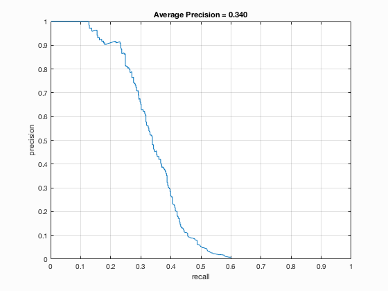
fig. 1 Average precision of multi-scale	fig. 2 HoG template from multi-scale


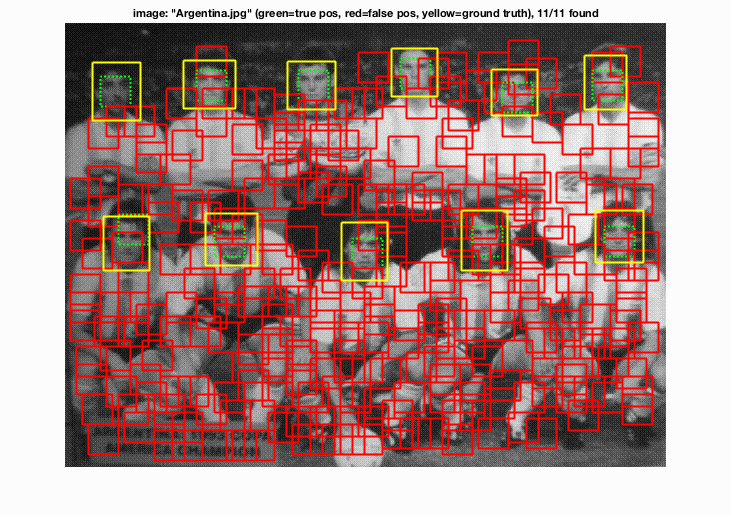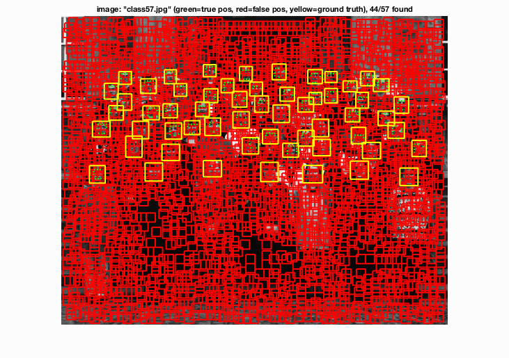
fig. 3 Single-scale performance on an image	fig. 4 Single-scale performance on an image

These are the single-scale results of the classifier. Average precision is 0.340 (34%). Since the threshold was so very low (-3), we get an extreme amount of red boxes cluttering the view. To my understanding, the number of red boxes really does not make much of a difference to the evaluation function, and only counts them as 'bad' if the confidence is too high for them. Since the AP is just about what we want it to be, we can say with sine certainty that these erroneous matches were of a very low confidence.

Multi-scale


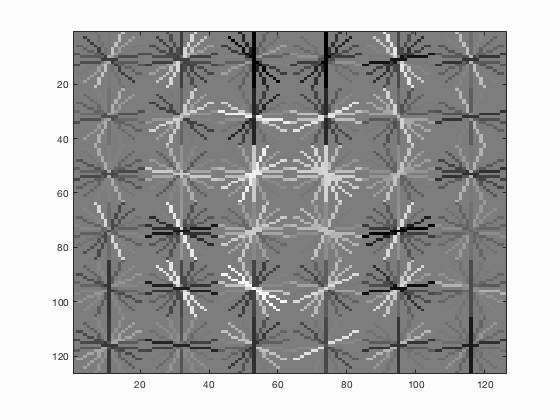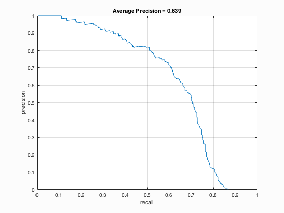
fig. 5 Average precision of multi-scale	fig. 6 HoG template


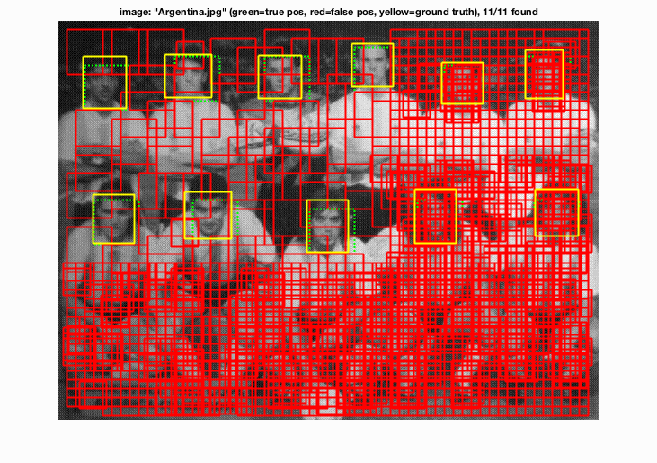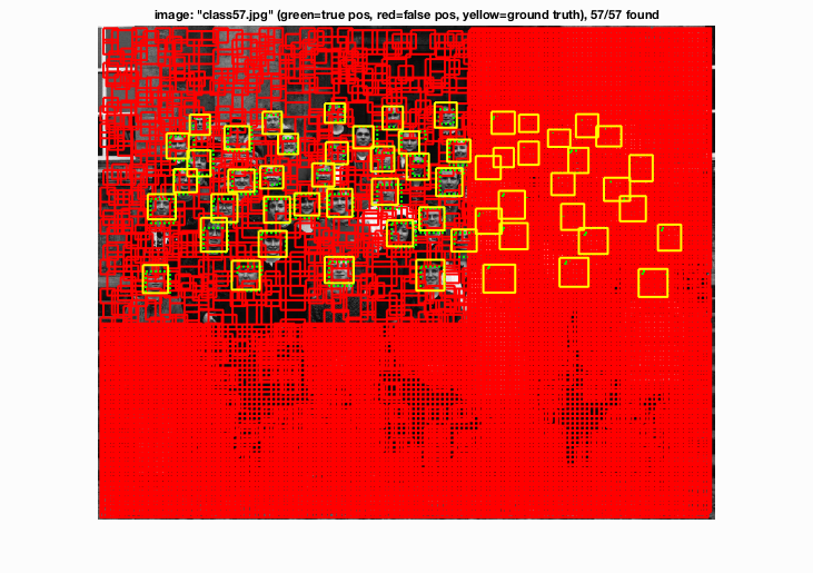
fig. 7 Multi-scale performance on an image	fig. 8 Multi-scale performance on an image

These are the multi-scale results of classifier. Average precision is .639 (63.9%). Again, low confidence => many red boxes. However, you can hopefully see that there are more green matches than before. Also note that, besides the increase in precision (almost double), there is an increase in recall. We can attribute both to the decreased granularity brought by analyzing the image at some lower scale.

Mitchell Manguno