Project 5 : Face Detection with a Sliding Window
Face detection
- Represent all training images as SIFT-like Histogram of Gradients.
- Training a linear SVM classifier (a HoG template)
- Classify images using sliding windows at multiple scales
Step 1. Load positive training crops and random negative examples
A. get_positive_features.m
Here we are given a series of faces which must be used to train our model as positive samples. We convert them to features by the following process.- Read images of size 36x36 images of faces
- Using vl_hog convert each image into a HoG template according to 'feature_params' where feature_params.template size is 36 (default) and feature_params.hog_cell_size size is 6 (default).
function features_pos = get_positive_features(train_path_pos, feature_params)

	image_files = dir(fullfile(train_path_pos, '*.jpg'));
	num_images = length(image_files);

	D = (feature_params.template_size/feature_params.hog_cell_size)^2 * 31;
	features_pos = zeros(num_images, D);

	train_path_pos = strcat(train_path_pos,'/');

	% read each image, compute the hog features and store it in features_pos
	for i = 1:num_images
	    image = im2single(imread(strcat(train_path_pos,image_files(i).name)));
	    image_hog = vl_hog(image, feature_params.hog_cell_size);
	    features_pos(i,:) = reshape(image_hog, 1 , D);
	end
end
B. get_random_negative_features.m
Here, we are given a series of images with no faces which must be used to train our model as negative samples. We convert them to features by repeating the process we followed for positive images. As we no not have fixed sized output of HoG of an image, we do extra computation to resize and convert it to the correct size. Images are also converted to grayscale because the positive training data is only available in grayscale.
function features_neg = get_random_negative_features(non_face_scn_path, feature_params, num_samples)

	image_files = dir(fullfile(non_face_scn_path, '*.jpg' ));
	num_images = length(image_files);
	non_face_scn_path = strcat(non_face_scn_path,'/');

	ratio_size = feature_params.template_size/feature_params.hog_cell_size;
	D = ratio_size^2 * 31;

	samples_per_image = ceil(num_samples/num_images);
	features_neg = zeros(samples_per_image*num_images,D);
	for i = 1:num_images
	    image = im2single(imread(strcat(non_face_scn_path,image_files(i).name)));
	    hog = vl_hog(image,feature_params.hog_cell_size);
	    [m,n,l] = size(hog);
	    m = m-rem(m,ratio_size);
	    n = n-rem(n,ratio_size);
	    resized = reshape(hog(1:m,1:n,:), (m*n*l)/D, D);
	    hog = datasample(resized, samples_per_image);
	    features_neg((i-1)*samples_per_image+1:i*samples_per_image,:) = hog;
	end
	features_neg = features_neg(1:num_samples, :);

end
Step 2. Train Classifier
We learn a single linear SVM as a detector. We define two variables, training_data and training_labels to hold the features and its corresponding labels. Both the positive and negative samples are combined at this step where the positive samples are given a label of 1 and negative samples are given a label of -1. vl_svmtrain uses this data to train a linear classifier. We can also set a regularization parameter(lambda) to ensure that we do not overfit/underfit our model and helps us control the amount of bias in the model. Here the value of lambda is set to 0.00001.
lambda = 0.00001;
training_data = [features_pos; features_neg];
training_labels = [ones(size(features_pos,1),1);ones(size(features_neg,1),1)*(-1)];
[w b] = vl_svmtrain(training_data',training_labels, lambda);
Step 3. Examine learned classifier
We first find the training error which must be extremely low (as it would imply that the model is well trained for the training images). We get the following results:
Initial classifier performance on train data:
  accuracy:   0.999
  true  positive rate: 0.401
  false positive rate: 0.000
  true  negative rate: 0.598
  false negative rate: 0.001
vl_hog: descriptor: [6 x 6 x 31]
vl_hog: glyph image: [126 x 126]
vl_hog: number of orientations: 9
vl_hog: variant: UOCTTI
Visualizing the learned detector using report_accuracy.m
The detector looks like an image (light regions represent high frequencies). This helps us understand what the classifier is trying to capture.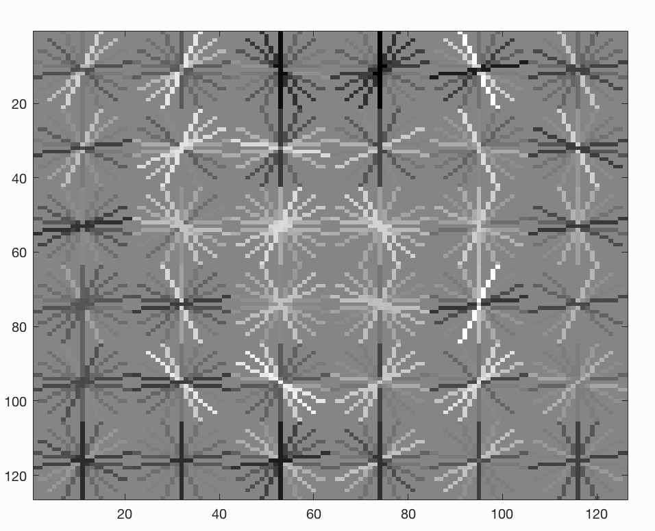
Visualizing the learned detector
Step 5. Run detector on test set.
We first convert each test image to a HoG feature space. We then step over the HoG cells taking groups of cells that are the same size as the template and classifying them. We use sliding windows at multiple scales, and if the classification is above a confidence of -1, we keep the detection and then pass all the detections for an image to a non-maximum suppression.
function [bboxes, confidences, imageids] = run_detector(test_scn_path, w, b, feature_params)

	test_scenes = dir(fullfile( test_scn_path, '*.jpg' ));
	ratio_size = feature_params.template_size / feature_params.hog_cell_size;
	D = ratio_size^2 * 31;
	iterations = 5;

	bboxes = [];
	confidences = [];
	imageids = {};

	for i = 1:length(test_scenes)
	    image = single(imread(fullfile(test_scn_path, test_scenes(i).name)))/255;
	    if(size(image, 3) > 1)
	        image = rgb2gray(image);
	    end

	    bboxes_image = [];
	    confidences_image = [];
	    imageids_image = {};

	    for j = 1:iterations
	        resize_factor = 0.8^(j-1);
	        hog = vl_hog(imresize(image,resize_factor),feature_params.hog_cell_size);
	        [m,n,~] = size(hog);
	        m = m - rem(m,ratio_size);
	        n = n - rem(n,ratio_size);

	        for k = 1:m-(ratio_size-1)
	            for l = 1:n-(ratio_size-1)
	                group_of_cells = hog(k:k+(ratio_size-1),l:l+(ratio_size-1),:);
	                classification = reshape(group_of_cells,1,D) * w + b;

	                if (classification > -1)
	                    x_min = (l*feature_params.hog_cell_size)-(feature_params.hog_cell_size-1);
	                    y_min = (k*feature_params.hog_cell_size)-(feature_params.hog_cell_size-1);
	                    bboxes_cell = [x_min, y_min, (x_min + feature_params.template_size), (y_min + feature_params.template_size)]./resize_factor;

	                    bboxes_image = [bboxes_image ; bboxes_cell];
	                    confidences_image = [confidences_image ; classification];
	                    imageids_image = [imageids_image ; {test_scenes(i).name}];
	                end
	            end
	        end
	    end

	    %non_max_supr_bbox can actually get somewhat slow with thousands of
	    %initial detections. You could pre-filter the detections by confidence,
	    %e.g. a detection with confidence -1.1 will probably never be
	    %meaningful. You probably _don't_ want to threshold at 0.0, though. You
	    %can get higher recall with a lower threshold. You don't need to modify
	    %anything in non_max_supr_bbox, but you can.
	    [is_maximum] = non_max_supr_bbox(bboxes_image, confidences_image, size(image));

	    confidences_image = confidences_image(is_maximum,:);
	    bboxes_image      = bboxes_image(is_maximum,:);
	    imageids_image   = imageids_image(is_maximum,:);

	    bboxes      = [bboxes;      bboxes_image];
	    confidences = [confidences; confidences_image];
	    imageids   = [imageids;   imageids_image];

	end
end
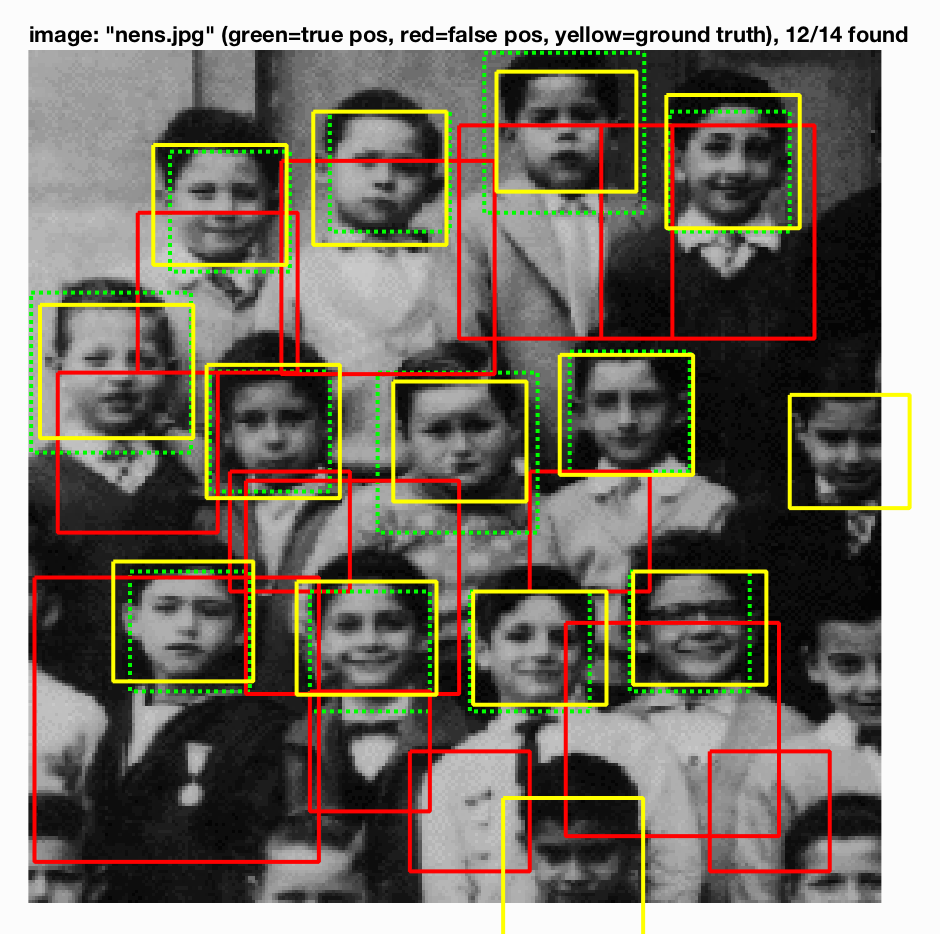
Step 6. Evaluate and Visualize detections.
We get an precision recall curve as follows for our final detector.

| Sample outputs | Analysis |
|---|---|
 |
Normal Sample Image with a single face |
 |
Normal Sample Image with a multiple faces |
 |
Image with a different face angle |
 |
Image in low intensity |
 |
Age insensitive |