Project 5 / Face Detection with a Sliding Window
In this project, the Dalal Triggs sliding window detector pipeline for face detection has been developed. Primary dataset used for this project was the CMU - MIT dataset provided. The HOG feature computation was performed using the vl_feat library. The report consists of the following sections
- Dalal Triggs pipeline implementation
- Extra credit - Hard negative mining
Dalal Triggs pipeline
The Dalal Triggs pipeline can be outlined as follows
- Extraction of HOG features from positive training data
- Extraction of HOG features from random negative training data
- Using the above training data, train a classifier like a linear SVM
- Perform sliding window detection over test set of images
HOG features were extracted using the vl_feat package. A number of parameters impacted the performance of the sliding window detector. Below is an analysis of how the performance improved with each free parameter's fine tuning The best average precision of 0.836 was achieved using a lambda parameter of 0.0001 (reasonable and doesn't overfit to the training data) - cross validated. Confidence threshold used in the detector in this case was 0.75.
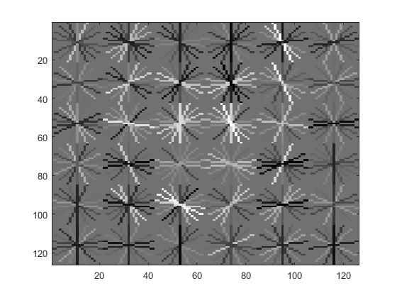
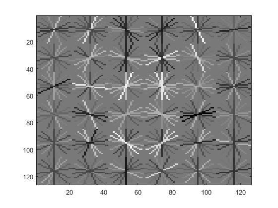
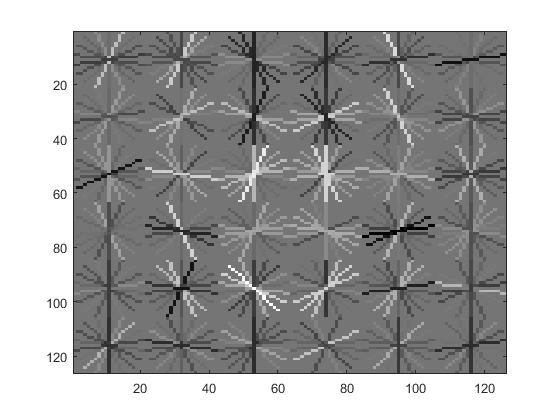
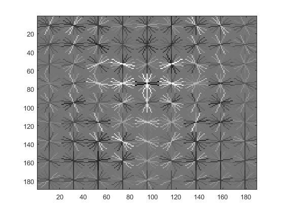
Face template HoG visualization for lambda 0.0001
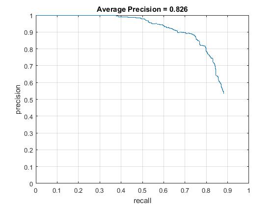
Precision Recall curve for confidence threshold of 0.75 and scales of order 0.9

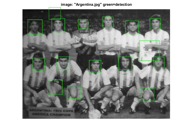
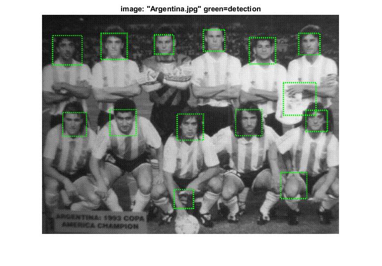
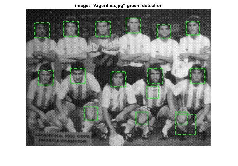
Detection on the test set for confidence threshold of 0.75
Scaling
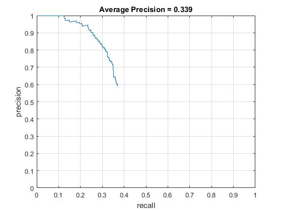
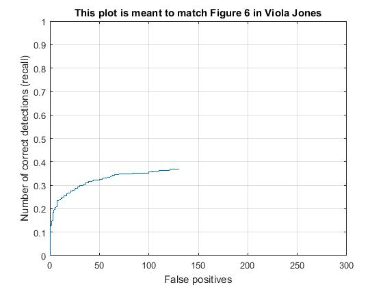
Scaling has a huge impact on the accuracy - Without scaling, average precision is a mere 0.339 . Supporting results are given below. Regularization param lambda 0.0001 and confidence threshold 0.75
|
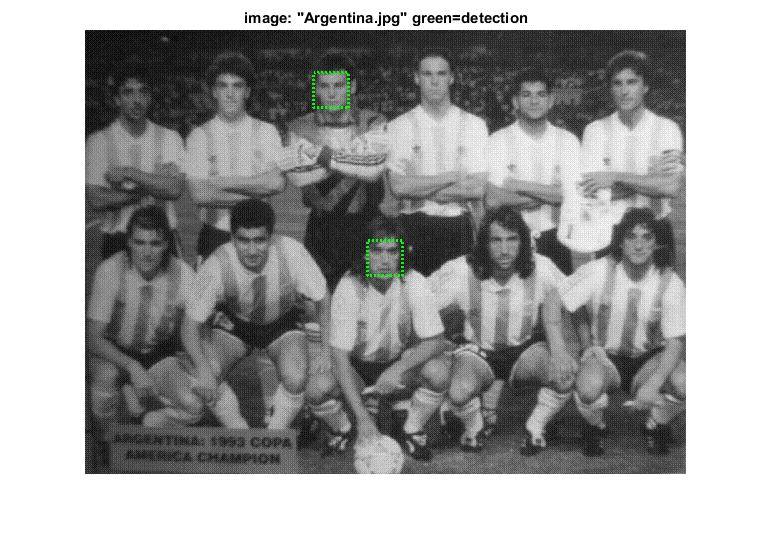
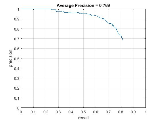
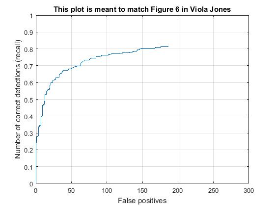
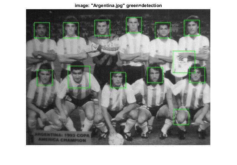
Scale of order 0.7, average precision increases to 0.769 . Supporting results are given below. Regularization param lambda 0.0001 and confidence threshold 0.75
|
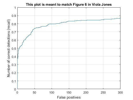
Scale of order 0.9, average precision increases to 0.821 . Supporting results are given below. Regularization param lambda 0.0001 and confidence threshold 0.75 Far better detection.
|
Hog Cell Size
While all the above tests were done for the default hog cell size of 6, a few trial runs on other hog cell sizes show that average precision improves with smaller hog cell sizes althought this causes the number of sliding windows evaluated to be much larger in number thereby considerably increasing the running time of the pipeline. Improves accuracy because granularity has been increased.
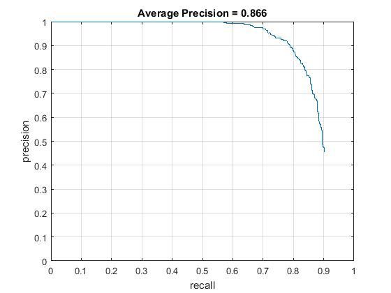
Hog cell size of 4, average precision increases to 0.866 . Supporting results are given below. Regularization param lambda 0.0001 and confidence threshold 0.75
|
Hog cell size of 2, average precision increases to 0.871 . Supporting results are given below. Regularization param lambda 0.0001 and confidence threshold 0.75
Confidence Threshold
Confidence threshold has proved to be a very effective and fairly tricky parameter to be tweaked. Making this threshold too strict / tight might reduce accuracy in terms of reducing the number of true positives detected. However relaxing this / making it too conservative is not too helpful as it allows false positives to sneak in. So depending on the desired / allowed percentage of false positives in requirements, this parameter can be tightened or relaxed. For the purpose of this report, the confidence thresholds of 0.4, 0.6 and 0.9 have been reported. 0.75 being the constant threshold in the above examples (hence not including as a separate entry for comparison here).
Confidence threshold of 0.4 Flipped values - true positive rate: 0.398 false positive rate: 0.001 true negative rate: 0.601, ap - 0.852
too many green boxes.
|
Confidence threshold of 0.9

|
Regularization parameter
This is again an interesting parameter to be tweaked. It is understandable that this parameter needs to be low since it is essentially a measure of how much you want to punish misclassifications i.e regularization parameter. However reducing this too far causes to overfit to the training dataset. While it is tempting to see a high accuracy with a low lambda, cross validation shows a huge error margin. For most of the report where best results are being reported, lambda has been calibrated at 0.0001. This was arrived at after multiple experimented values. For this project, attempted lambdas of 0.1, 0.01, 0.05, 0.001
Extra credit
Hard negative mining done 2 ways
Hard negative mining is implemented using a hard upper bouond on the negative examples being made available to the training phase of the classifier. Once the classifier has been trained, we use the training set itself in the pseudo-test phase, pick all the features which continue to get falsely classified as a face and push them back as negative examples in the training set. Using this new training set, we re-train the classifier. The performance improvement is considerable only when this is done as an iterative process. number of iterations over which hard negatives are mined has been varied from 1-8. I have left it at 8 in the commented out section. Without repeated retraining of the classifier, in the case of frontal faces, the improvement in average precision is very modest and not worth the hard negative mining phase. Also as suggested in the instructions, this is useful only if we have an upper bound on the number of negatives we make available in the trianing phase. Reduction in the number of false positives is not that great.
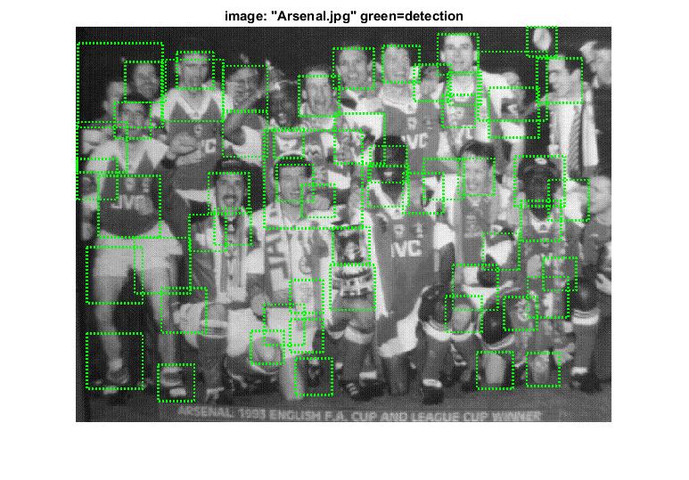
HNM in comparsion to the best achieved thus far - i.e. 0.825 with 10000 negatives, 0.75 threshold, and 0.0001 regularization.
HNM achieves average precision at par (0.816) with this score with just 5000 negatives, threshold of 0.65 while mining hard negatives and retaining the same regularization parameters. The number of iterations for this is 8
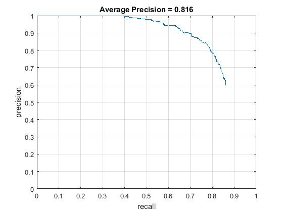
Precision Recall curve
Another way of getting Hard negatives - data set dependant
Hard negative mining seems to give better performance if all negative examples in the dataset are mined for hard negatives i.e run detector on all negatives available instead of sampling number_of_samples (all images instead of 10000 or upper bound 5000 as in previous approach) - Treat them as hard negatives and re train the classifier only once. Surpsingly this gives better improvement - about 0.863 (in comparison to 0.83 range) when this is done. However I think this is too specific to the data set at hand and might be overfitting to the negatives present in the dataset.
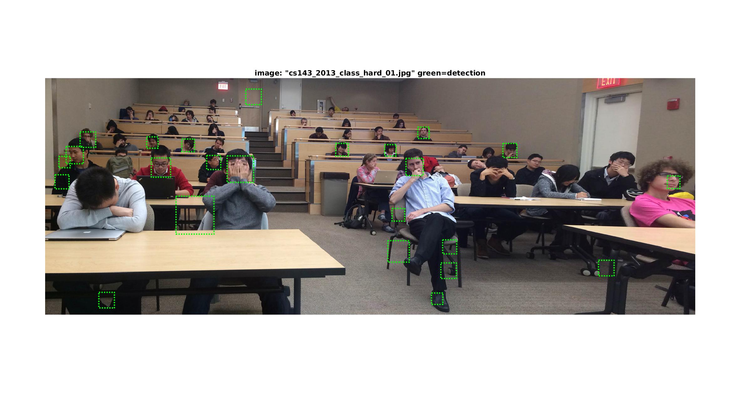
Test scenes for the class images
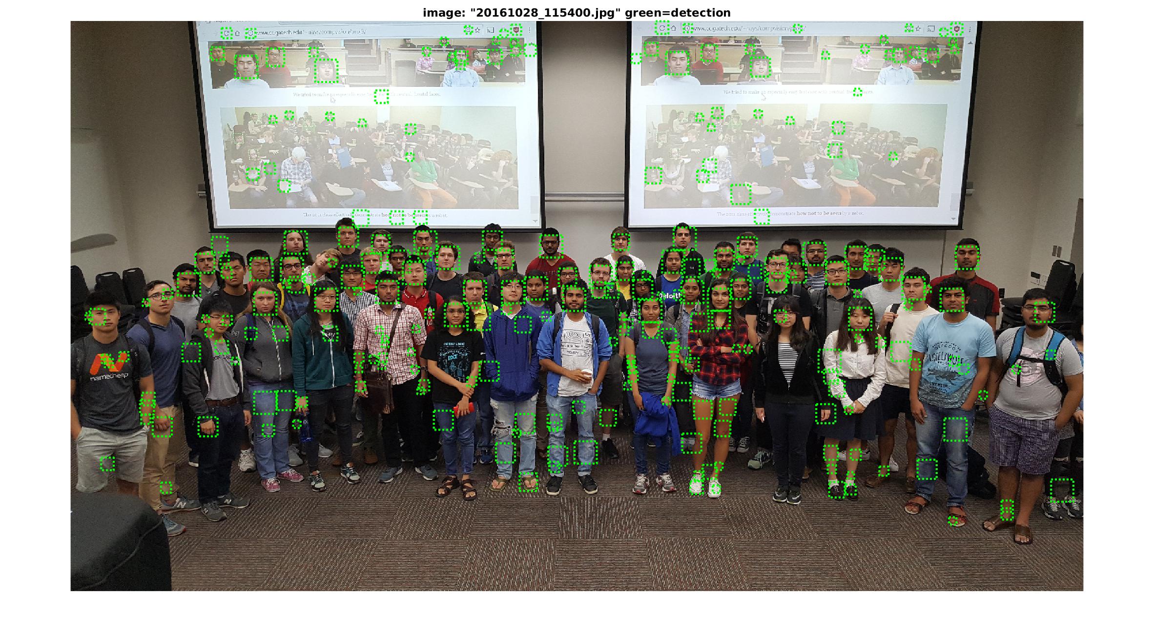
Observation - too many positives detected however a good number of accurate faces detected as well.
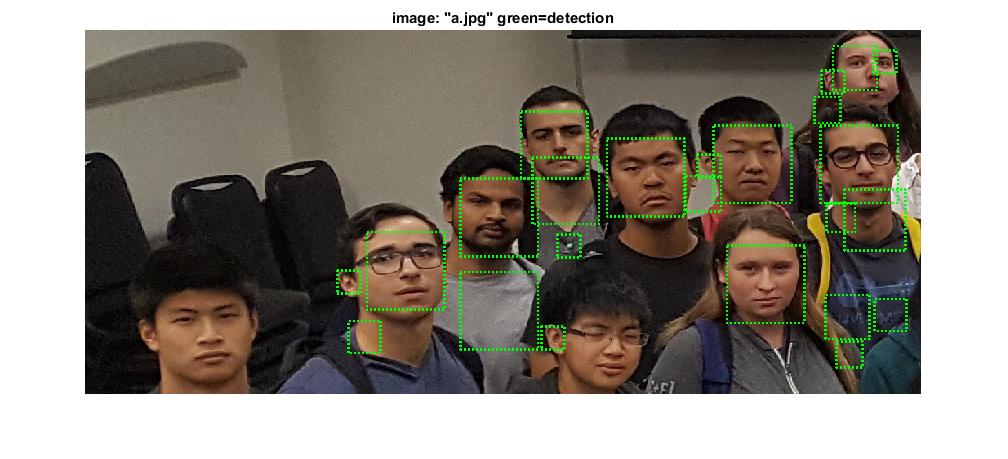
Experimenting with scale - using an upscaled snip of one part of the image - Shows face detected for a face that was missed out in the previous detection - Not enough scales in the code since the PASCAL VOC dataset did not have so many scales. Also might have given better detection if I had tried upscaling as well. I have kept it as a todo for now.
With obscuring - Some faces partially obscured have still been detected - Possible improvement by reducing the hog cell size. Here the default hog cell size 6 has been used.