Nitin Kodialbail

Extract HOG features from positive and negative training images

The positive images consist of images of cropped faces of size 36x36. 36x36 is the template size to extract HOG features from. So each image generates hog features of size 6x6x31. This matrix is reshaped as a feature vector and is stored in a row of a matrix called 'features_pos'. Finally the 'features_pos' matrix will have features of all the positive train images stored row wise.

For the negative train images, images of size 36x36 are randomly cropped from each negative image and their hog feature vectors are stored in rows of a matrix called 'features_neg'. Multiple images are cropped from each negative train image such that we finally end with up 5000 negative HOG feature vectors in 'features_neg'.

Train Linear SVM classifier using the HOG features extracted

The positive features are labelled as +1, while the negative features are labelled as -1. A linear SVM classifier is trained using these positive and negative features. Regularization parameter is kept as 0.0001 to prevent overfitting to training data.

Build multi scale sliding window detector to find faces in test images using the classifier

Here each test image is converted to its hog feature space. Initially in the detection of faces in the test images, the sliding window is run on a single scale, i.e the original image scale. The stride of the sliding window is set to 1 for highest accuracy at the cost of slower run time. Each window of the hog feature space is classified by the linear classifier as a face or not. The classifier returns a confidence value of the window being a face. A confidence threshold of -1.0 is used in order to classify any window of the image whose confidence is above that, as a face. This gives us an average precision value of 0.406.

Next, multi scale sliding window is implemented. Here each image is repeatedly downsized by a fixed factor of 0.7 and then each downscaled image is converted to its hog feature space. The sliding window is then run on each of these hog feature spaces. The co-ordinates of any window which is detected as a face by the classifier is noted and its equivalent co-ordinates in the original image scale is found out. Again a confidence threshold of -1.0 is used in order to filter out the windows not having a face. With multi scale detection added, the average precision value increases to 0.846. The downscaling is stopped when the hog feature space of the image is smaller than the size of the sliding window.

When the mirror image of the positive images are added to the original set of positive images, in order to augment the positive dataset, we get an average precision value of 0.851, using the same parameters used previously. The increase in average precision is not significant. The mirror images can be used in the case of face detection as faces are symmetrical.

When the downsize factor is increased from 0.7 to 0.9, we get an average precision value of 0.895, while keeping the remaining parameters same as before. Therefore, the increase in number of scales of the images gave better precision.

Bells and Whistles: Implement hard negative mining

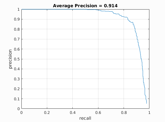
The trained linear SVM classifier is run on the negative train dataset with the help of multiscale sliding window. The detections which are obtained are the false positives which are not actually faces. These detections are cropped out of the negative train images and they are resized to hog template size of 36x36 and then they are converted to hog features of size 6x6x31. These hog feature matrices are converted to vectors and appended as additional rows to 'features_neg' matrix. Therefore the number of negative features increase and then the classifier is retrained again with this new negative feature set. This classifier can again be run on negative training dataset and the above procedure can be run again and again in cycles until the desired number of hard negative features are obtained. Finally after we are satisfied with the mining of hard negative features, we use the final trained classifier on the test data set. But in the trials which were ran, hard negative mining improved the average precision only slightly. i.e I used 10000 hard negatives instead of random negatives and trained only these hard negatives against the positives and built an SVM classifier. This classifier when run on the test dataset gave an average precision of 0.914 which is a slight increase from the previous value of 0.895.

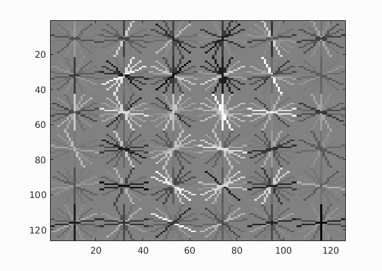
Face template HoG visualization for the starter code. Hog cell size used = 6

Precision Recall curve for the starter code.

Example of detection on the test set from the starter code with confidence threshold = -1.

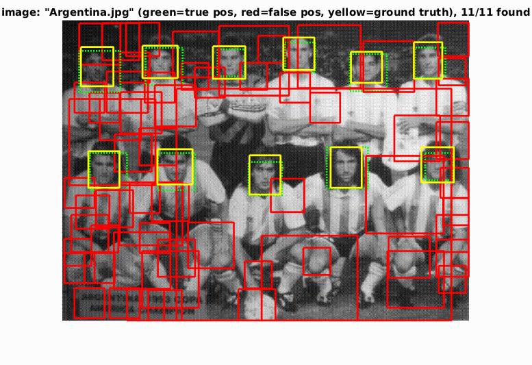
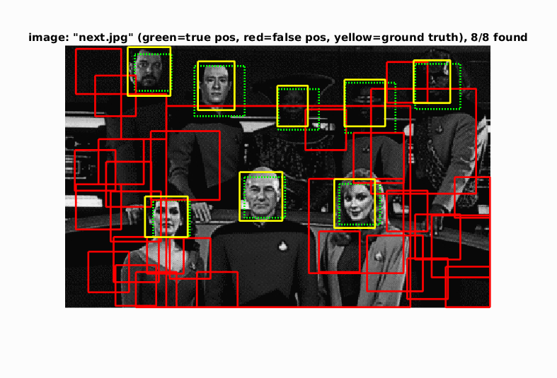
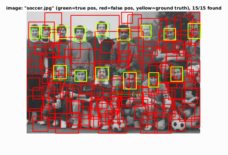
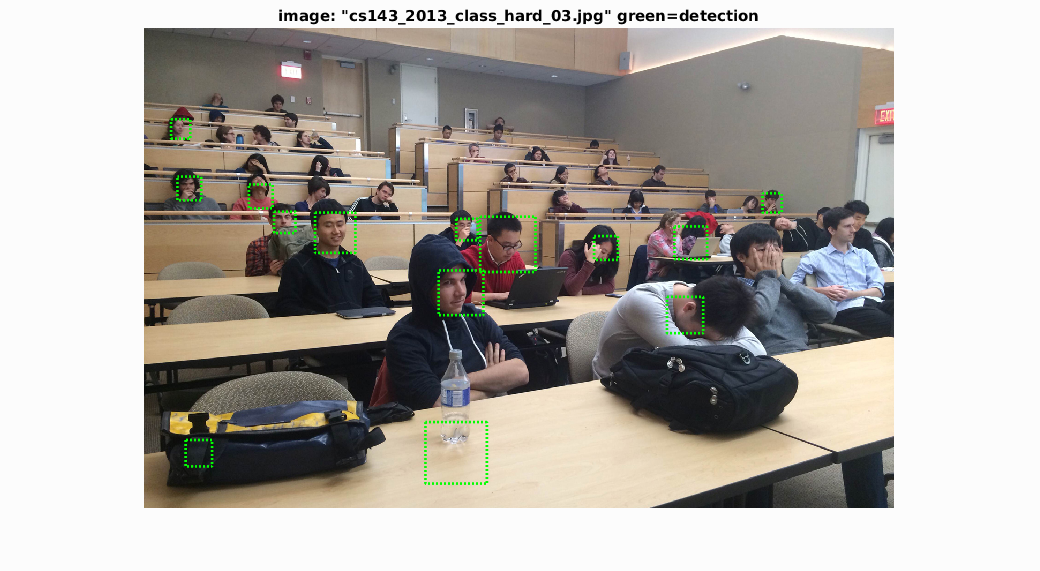
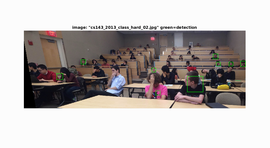
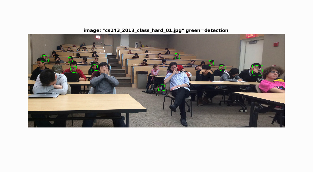
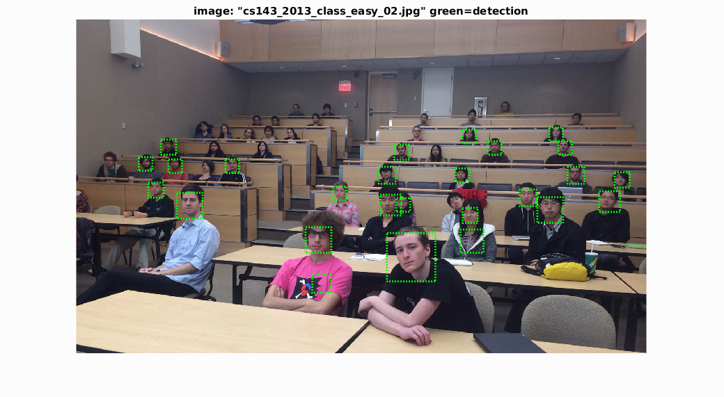
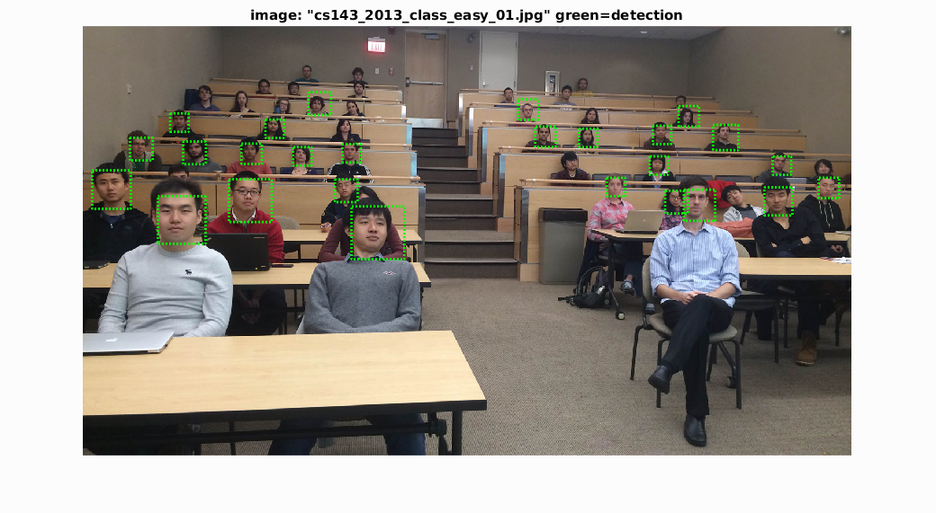
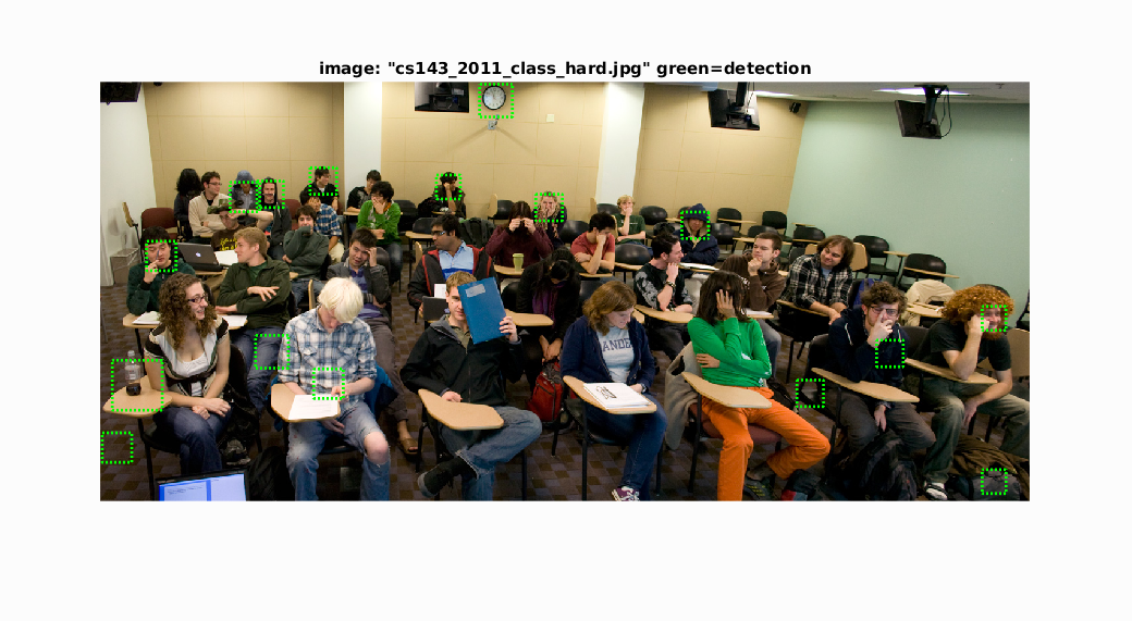
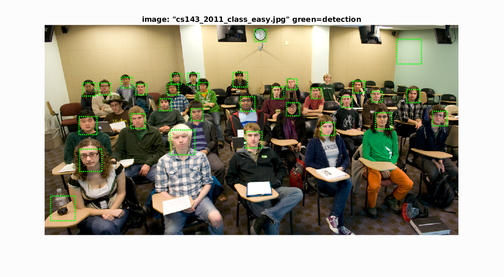
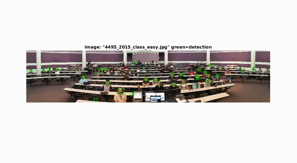
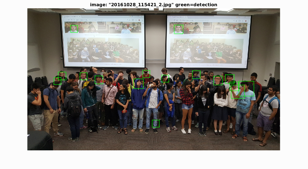
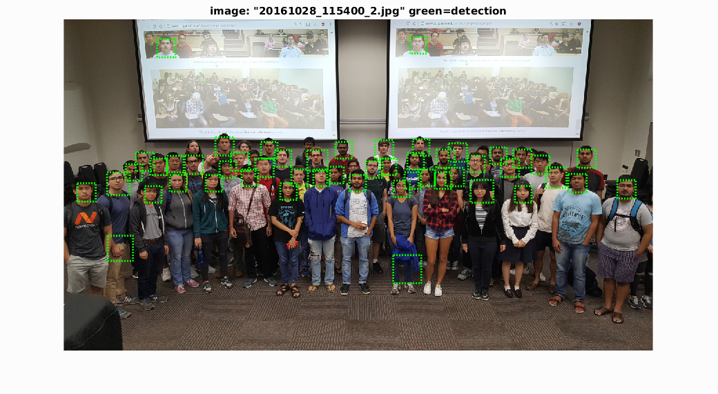
Example of detections on class images with confidence threshold = +1