Project 5 / Face Detection with a Sliding Window
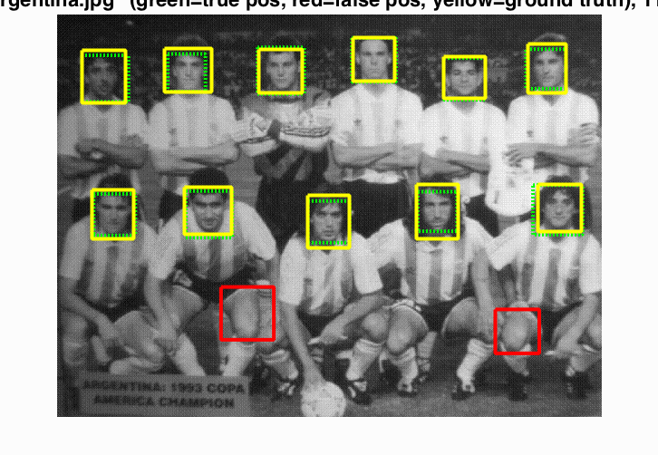
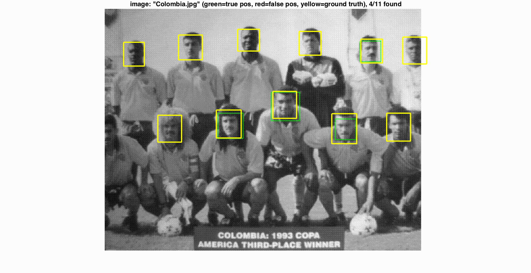
Face detection on Argentenian Football team. 11/11 faces found with 2 false positives
In this project we used the Dalal-Triggs method to implement face detection suing a training set from Caltech and random test images from and MIT+CMU test set. The basic pipeline follows this process:
- Load positive training images
- Load random negative images
- Select the number of negative examples
- Train an svm classifier with the positive and negative training examples.
- Run test examples with the trained linear classifier from the previous step
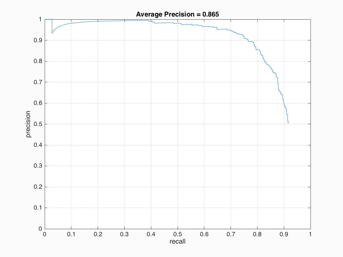
My average precision was 0.865.
Linear Classifier
get_positive_features and get_random_negative_features convert samples passed into a histogram of gradients format using vl_hog. get_positive_features uses the caltech dataset to retrieve faces from. get_random_negative_features retrieves num_samples random negative features from the test set. I found that a combination of a higher number of samples and striciter confidence score provided a higher average precision. I initially started with just 1 scale for random negative features and had an average training accuracy of about 0.782. After doing this at multiple scales, I have an average training accuracy of 0.999, false positive rate of 0, and true negative rate of 0.817. I choose to do 5 scales per image. At first I was doing scales: [0.20, 0.40, 0.60, 0.80, 1.0] for each image but found that selecting the scale randomly worked slightly better. 0.990 accuracy for determined scales vs 0.999 for random scales. I'm using 30000 random negative samples in my implementation of the project. For the svm classifier, a lambda of 0.0001 works the best. The hog template is shown below.
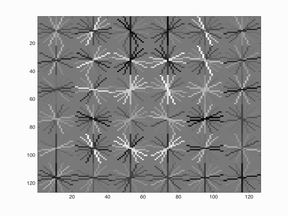
Hog template. If you look at it from a distance or make it smaller, you can see the basic outline of a face including eyes and a mouth.
Run_detector
Run_detector converts each test image to a HoG feature space. Then I step over the HOG cells, classify the cells, and perform non maximum supressions. This process is performed on multiple scales (roughly 7 per image). The cell size I chose to submit this project with is 6. I found it to be very fast (1-2 minutes) and have reasonable precision 0.865. However, with a cell size of 4 and more so 3, the average precision did go slightly up. With a cell size of 3 I saw average precision hovering around 0.9. However, these two cell sizes turned out to run extremely slow (> 10 minutes). After grouping the cells, I apply the trained linear classifiers parameters and select the ones with above a certain confidence. Initially, I had a confidence greater than 0.73 with 10000 random negative examples which resulted in an average precision of 0.81. However, increasing the number of random negative examples and raising the confidence bar, in general, resulted in higher average precisions. I found a confidence greater than 0.80 to work the best. Anything less than that results in too many false positives and lower average precision. The code in figure 1 highlights the core of the sliding window detector. Precision vs recall graph is shown below. As the number of relevant items selected goes up, the precision goes down which is expected.
Parameters Chosen
Figure 1
% Sliding window code
for x=1:x_window
    for y=1:y_window
        p = hog(y:y+pix_per_cell - 1, x:x+pix_per_cell-1, :);
        window = reshape(p, 1, pix_per_cell^2 * 31);
        windows((y_window)*(x-1)+y, :) = window;
    end
end

% Pass through linear classifier and take most confident matches
cur_score = b + windows*w;
thresholded_indices = find(cur_score > threshold);
confidence = cur_score(thresholded_indices);
Results in a table
|
|