Project 5 / Face Detection with a Sliding Window
In this project, I implemented a sliding window classifier using a histogram of gradients (HOG) feature representation. As a baseline, I trained an SVM on a moderate amount of positive examples and a large amount of negative examples. I then implemented hard negative mining to augment a small amount of negative examples with more difficult examples. Finally, I used a fully connected neural network instead of an SVM to get a nonlinear classifier from the HOG features.
Positive and negative features
For both positive and negative images, I run vl_hog. For the negative images, I extract random HOG patches. The code for both functions is shown below.
function features_pos = get_positive_features(train_path_pos, feature_params)

image_files = dir( fullfile( train_path_pos, '*.jpg') ); %Caltech Faces stored as .jpg
num_images = length(image_files);

template_size = feature_params.template_size;
hog_cell_size = feature_params.hog_cell_size;

feature_dim = (template_size / hog_cell_size)^2 * 31;

features_pos = zeros(num_images, feature_dim);
for i = 1:num_images
    file_path = fullfile(train_path_pos, image_files(i).name);
    img = single(imresize(imread(file_path), [template_size, template_size]))/255;

    hog = vl_hog(img, hog_cell_size);
    features_pos(i,:) = hog(:);
end
function features_neg = get_random_negative_features(non_face_scn_path, feature_params, num_samples)

image_files = dir( fullfile( non_face_scn_path, '*.jpg' ));
num_images = length(image_files);

template_size = feature_params.template_size;
hog_cell_size = feature_params.hog_cell_size;

feature_dim = (template_size / hog_cell_size)^2 * 31;
features_neg = zeros(num_samples, feature_dim);

for i = 1:num_samples
    file_path = fullfile(non_face_scn_path, image_files(randi(num_images)).name);
    img = single(rgb2gray(imread(file_path)))/255;
    [rows, cols, ~] = size(img);
    row_end = rows - template_size + 1;
    col_end = cols - template_size + 1;

    sampled_rows = randi(row_end) + (0:template_size-1);
    sampled_cols = randi(col_end) + (0:template_size-1);

    img_patch = img(sampled_rows, sampled_cols, :);
    hog = vl_hog(img_patch, hog_cell_size);
    features_neg(i,:) = hog(:);
end

end
Training SVM
Given the positive and negative features, I then train the SVM detector.
function [svm_fn, w, b] = train_svm(features_pos, features_neg, lambda)

if nargin == 2
    lambda = 1e-4;
end

features = [features_pos; features_neg]';

num_positive = size(features_pos, 1);
num_negative = size(features_neg, 1);
labels = [ones(num_positive, 1); -ones(num_negative, 1)];

[w, b] = vl_svmtrain(features, labels, lambda);
svm_fn = @(features) features*w + b;

end
Running detector
For each test image, I loop over different scales, resizing the image to each scale. For each scaled image, I compute the HOG features and run the detector on it. For each confidence above a certain threshold, I put a bounding box on the corresponding feature. I then run non_max_supr_bbox to remove overlapping bounding boxes. The code is shown below.
function [bboxes, confidences, image_ids] = ....
    run_detector(test_scn_path, classifier_fn, feature_params, detection_params)

test_scenes = dir( fullfile( test_scn_path, '*.jpg' ));

%initialize these as empty and incrementally expand them.
bboxes = zeros(0,4);
confidences = zeros(0,1);
image_ids = cell(0,1);

threshold = detection_params.threshold;
scale_factor = detection_params.scale_factor;
num_scales = detection_params.num_scales;

for i = 1:length(test_scenes)

    fprintf('Detecting faces in %s\n', test_scenes(i).name)
    img = imread( fullfile( test_scn_path, test_scenes(i).name ));
    img = single(img)/255;
    if(size(img,3) > 1)
        img = rgb2gray(img);
    end

    cur_bboxes = zeros(0,4);
    cur_confidences = zeros(0,1);
    for j = 0:num_scales-1
        [cur_bboxes_level, cur_confidences_level] = find_bboxes(img, ...
            feature_params, classifier_fn, threshold, scale_factor^j);
        cur_bboxes = cat(1, cur_bboxes, cur_bboxes_level);
        cur_confidences = cat(1, cur_confidences, cur_confidences_level);
    end
    cur_image_ids = repmat({test_scenes(i).name}, size(cur_bboxes,1), 1);

    %non_max_supr_bbox can actually get somewhat slow with thousands of
    %initial detections. You could pre-filter the detections by confidence,
    %e.g. a detection with confidence -1.1 will probably never be
    %meaningful. You probably _don't_ want to threshold at 0.0, though. You
    %can get higher recall with a lower threshold. You don't need to modify
    %anything in non_max_supr_bbox, but you can.
    [is_maximum] = non_max_supr_bbox(cur_bboxes, cur_confidences, size(img));

    cur_confidences = cur_confidences(is_maximum,:);
    cur_bboxes      = cur_bboxes(     is_maximum,:);
    cur_image_ids   = cur_image_ids(  is_maximum,:);

    bboxes      = [bboxes;      cur_bboxes];
    confidences = [confidences; cur_confidences];
    image_ids   = [image_ids;   cur_image_ids];
end

end

function [bboxes, confidences] = find_bboxes(img, feature_params, ...
    classifier_fn, score_threshold, scale_factor)

img = imresize(img, scale_factor, 'bilinear');

template_size = feature_params.template_size;
hog_cell_size = feature_params.hog_cell_size;
[features, size_x, size_y] = form_hog_features(img, template_size, ...
    hog_cell_size);
scores = classifier_fn(features);
is_face = (scores >= score_threshold);
confidences = scores(is_face);

bboxes = zeros(0, 4);
indices = 1:size(features, 1);
for i = indices(is_face)
    [x, y] = ind2sub([size_x, size_y], i);
    x_min = hog_cell_size*(x-1)/scale_factor + 1;
    y_min = hog_cell_size*(y-1)/scale_factor + 1;
    x_max = x_min + template_size/scale_factor - 1;
    y_max = y_min + template_size/scale_factor - 1;
    bboxes = cat(1, bboxes, [x_min, y_min, x_max, y_max]);
end

end

function [hog_features, size_x, size_y] = ...
        form_hog_features(img, template_size, hog_cell_size)

hog = vl_hog(img, hog_cell_size);
patch_width = template_size / hog_cell_size;
feature_dim = patch_width^2 * 31;
size_x = size(hog,2) - patch_width + 1;
size_y = size(hog,1) - patch_width + 1;
hog_features = zeros(size_x*size_y, feature_dim);
for x = 1:size_x
    for y = 1:size_y
        hog_patch = hog(y + (0:patch_width-1), x + (0:patch_width-1), :);
        hog_features(x + size_x*(y-1),:) = hog_patch(:);
    end
end

end
Results
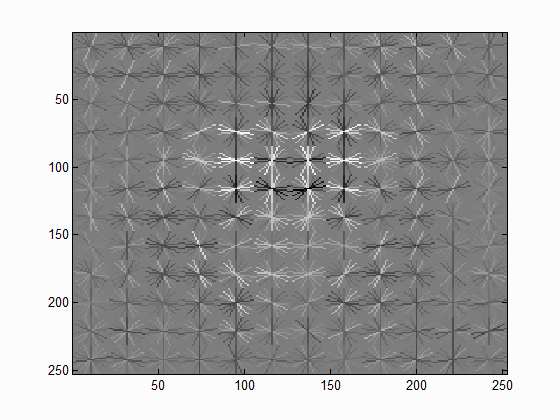
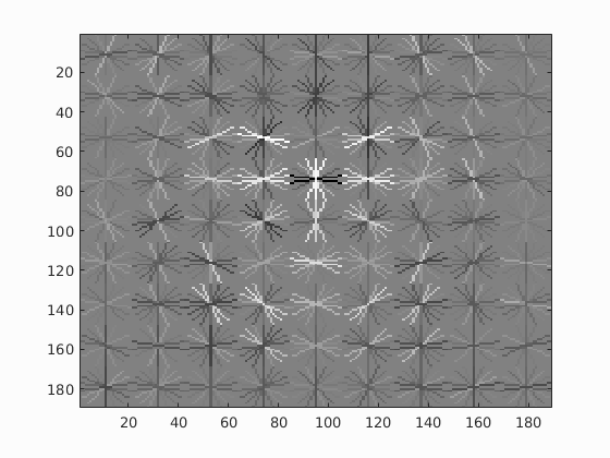
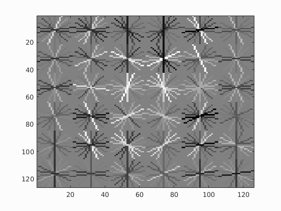
I randomly sampled 100,000 negative examples and had the template size set to 36-by-36 pixels. I varied the HOG cell size to see how it changed the visualization of the SVM. Below are the visualizations of the SVM with cell sizes of 3, 4, and 6 pixels, respectively. All of these seem to positively weight features like eyes, the nose, and the general outline of the head. This is best seen in the smaller images just below. However, the SVM with a cell size of 3 seems to weight features on a finer scale. To achieve the highest accuracy, this was the cell size I used for testing.
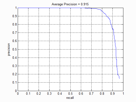
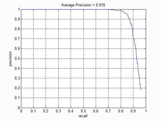
For the multi-scale detector, I extracted HOG features over 15 scales with a scaling factor of 0.9 (meaning that the features are found down to about one-quarter the size of the original image). The recall-precision curve for the SVM with a cell size of 3 is shown below. To keep the classifier from returning too many false positive, I set the activation threshold to 0.8. With this threshold, I was able to achieve an average precision of 89.7%, precision of about 80%, and recall of about 90%.
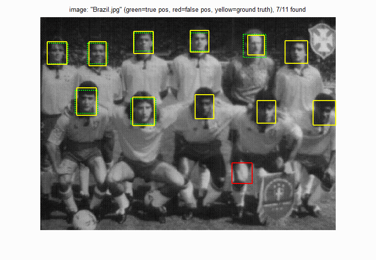
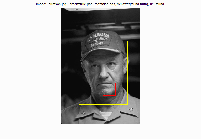
Some example detections are shown below. With the crowd of students, the SVM can detect all but one of the students and produces six false positives. On the Brazil photo, the SVM struggles a bit more, possible because the faces are a bit obscured and blurry. On the Crimson Tide photo, the SVM cannot detect Gene Hackman, even though his face is in clear view. This is probably because the image is too large, even when scaled to one-quarter size.

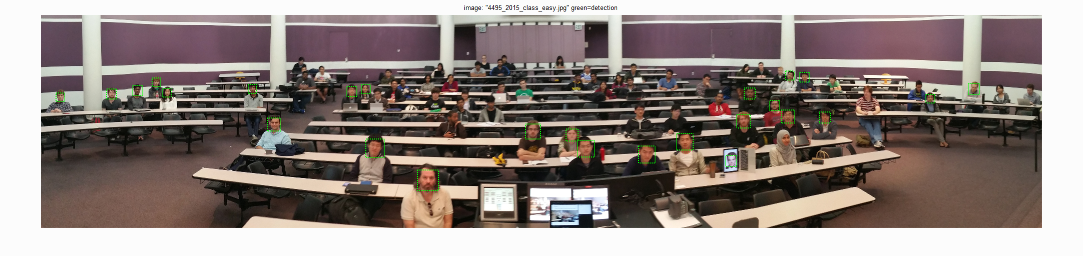
I also ran the detector on the class images. For the CS 4996 class, it mostly detects people in the front rows and fails to detect people in the back row. This is probably because the faces in the back are too small to detect. For the CS 143 easy image, it again detects people in the front but not in the back of the class. For the hard image, the SVM has a really difficult time finding heads, only detecting those that are mostly unobscured.


Extra credit: Hard negative mining
I also implemented hard negative mining. After training the classifier with a small number of negative examples, I loop over every negative training image and extract patches that score above the the classifier threshold. Afterwards, those negative features are added to the smaller set of negative features to train a more robust classifier.
function features_hard_neg = get_hard_negative_features(non_face_scn_path, ...
    classifier, feature_params, detection_params)

[bboxes, confidences, image_ids] = run_detector(non_face_scn_path, ...
    classifier, feature_params, detection_params);
bboxes = round(bboxes);

template_size = feature_params.template_size;
hog_cell_size = feature_params.hog_cell_size;

feature_dim = (template_size / hog_cell_size)^2 * 31;
num_negative = length(confidences);
features_hard_neg = zeros(num_negative, feature_dim);
for i = 1:num_negative
    x_min = bboxes(i,1);
    y_min = bboxes(i,2);
    x_max = bboxes(i,3);
    y_max = bboxes(i,4);

    img_full = rgb2gray(imread(fullfile(non_face_scn_path, image_ids{i})));

    if x_min < 1 || y_min < 1 || x_max > size(img_full, 2) || y_max > size(img_full, 1)
        continue;
    end

    img_patch = imresize(img_full(y_min:y_max, x_min:x_max), ...
        [template_size, template_size]);
    img_patch = single(img_patch)/255;

    hog = vl_hog(img_patch, hog_cell_size);
    features_hard_neg(i,:) = hog(:);
end

end
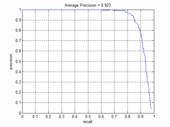
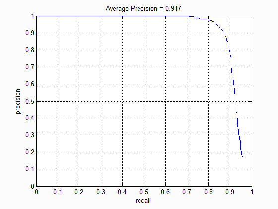
Before hard negative mining, I train the SVM with all the positive examples and 5,000 random negative examples. After running hard negative mining, I extract 13,520 additional hard negative examples. However, even adding these examples don't affect the SVM's performance much. The recall-precision curve at the left corresponds to the SVM trained with only 5,000 examples while the one on the right corresponds to the SVM trained with both the 5,000 negative examples and the hard negative examples. Both curves look quite identical, implying that face detection with a linear classifier only requires a small number of random negative examples rather than "difficult" negative examples.
Extra credit: Neural net with HOG inputs
I also used MATLAB's neural network toolbox to train a non-linear classifier of the HOG features. The network I used has two layers with the hidden layer having 100 units and the tanh nonlinearity.
function [classifier, net, tr] = train_net(features_pos, features_neg)

features = [features_pos; features_neg]';
num_positive = size(features_pos, 1);
num_negative = size(features_neg, 1);
labels = [repmat([1; 0], 1, num_positive), repmat([0; 1], 1, num_negative)];

net = patternnet(100);
[net, tr] = train(net, features, labels);

classifier = @classifier_fn;

    function scores = classifier_fn(features)
        probs = net(features');
        scores = prob_to_score(probs(1, :))';
    end

end
The resulting precision-recall curve again looks quite similar to the previous recall-precision curves. It does, however, seem that the neural network performs a little bit worse, seeing as it falls below 100% recall and 80% precision sooner. This could be because of some overfitting since both the SVM and neural networks achieve about 100% accuracy on the training set. Thus, it might make more sense to use the neural network if more training data is available.