Project 5 / Face Detection with a Sliding Window
Face HoG Visualization
Overview
The project uses Matlab to perform Face Detection with a sliding window. By training over sets explicitly containing faces and explicitly not containing faces, we use a SVM to obtain a classifier. This classifer is then used with a sliding window approach to attempt to detect faces in images.
Algorithms
Get Positive Features
The get positive features algorithm returns positive features (faces) from training data. We use vl_hog to create a histogram of gradients for feature detection. The details are summarized below:
- Load all images in training data directory
- For each image, load the image data and convert to a single precision struct
- Use vl_hog to create a histogram of gradients with a supplied cell size
- Reshape the histogram to be a column vector and append to our positive features matrix
Get Random Negative Features
The get random negative features algorithm returns negative random features (non-faces) from training data. The images are transformed to grayscale from rgb to match the positive training data that is grayscale. We use vl_hog to create a histogram of gradients for feature detection. The details are summarized below:
- Load all images in training data directory
- Determine number of samples per image based on the number of samples parameter
- For each image, load the image data and convert to a grayscale image
- Collect n random samples for the image, where n is the number of samples per image
- For each random sample, use matlab's RAND to get a random X and Y coordinate
- Cut a random feature subimage based on the above X and Y of size template_size
- Perform vl_hog on this subimage to obtain a histogram of gradients
- Reshape the histogram to be a column vector and append to our positive features matrix
Classifier Training
The classifier training algorithm use's vl_svmtrain to train an SVM classifier on the training features. By using the results of Get_Positive_Features and Get_Random_Negative_Features, we can create a label vector containg +1 and -1 for the results. We feed this into vl_svmtrain to train the classifier along with a predefined lambda value for regularization
- Append positive and negative training features to create X
- Calculate length of postive and negative training feature matrices
- Combine these lengths to create a label vector
- Assign a value of +1 to positive training instances and -1 to negative instances.
- Pass X, the labels, and a constant lambda (regularization) value into vl_svmtrain to train the classifier
Run Detector
The run detector algorithm returns face detections from a set of input test images. The images are transformed to grayscale to match training data. For each image, we start at its original scale and then scale down by a constant scale factor until it is smaller than the template size. We use vl_hog to create a histogram of gradients for face detection. If a detection passes a given detection threshold, it is considered a positive match and returned as such. The details are summarized below:
- Load all images in test data directory
- For each image, convert to grayscale if necessary
- While the image size is greater than the template_size constant:
- -Perform vl_hog on the image to get a histogram of gradients
- -Determine maximum number of vertical and horizontal windows
- -Slide over each window and take the vl_hog subhistogram
- -Apply the classifier to the subhistograms
- -If classification confidence is above a constant threshold, add a positive result and bounding box to results
- -Scale image down by a constant scale factor
- Perform non-maximum supression on bounding boxes and confidences
Decisions & Results
This project required a variety of parameter tuning to obtain optimal results.
| Paramater | Value |
| Template size | 36 |
| Cell Size | 3 |
| Lambda | 0.0001 |
| Detector Image Scale Constant | 0.9 |
| Confidence Threshold | 0.7 |
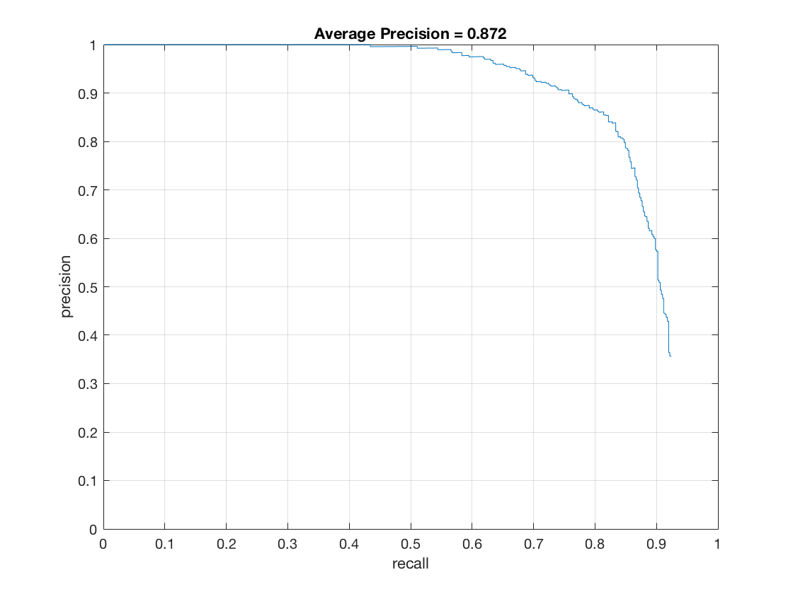
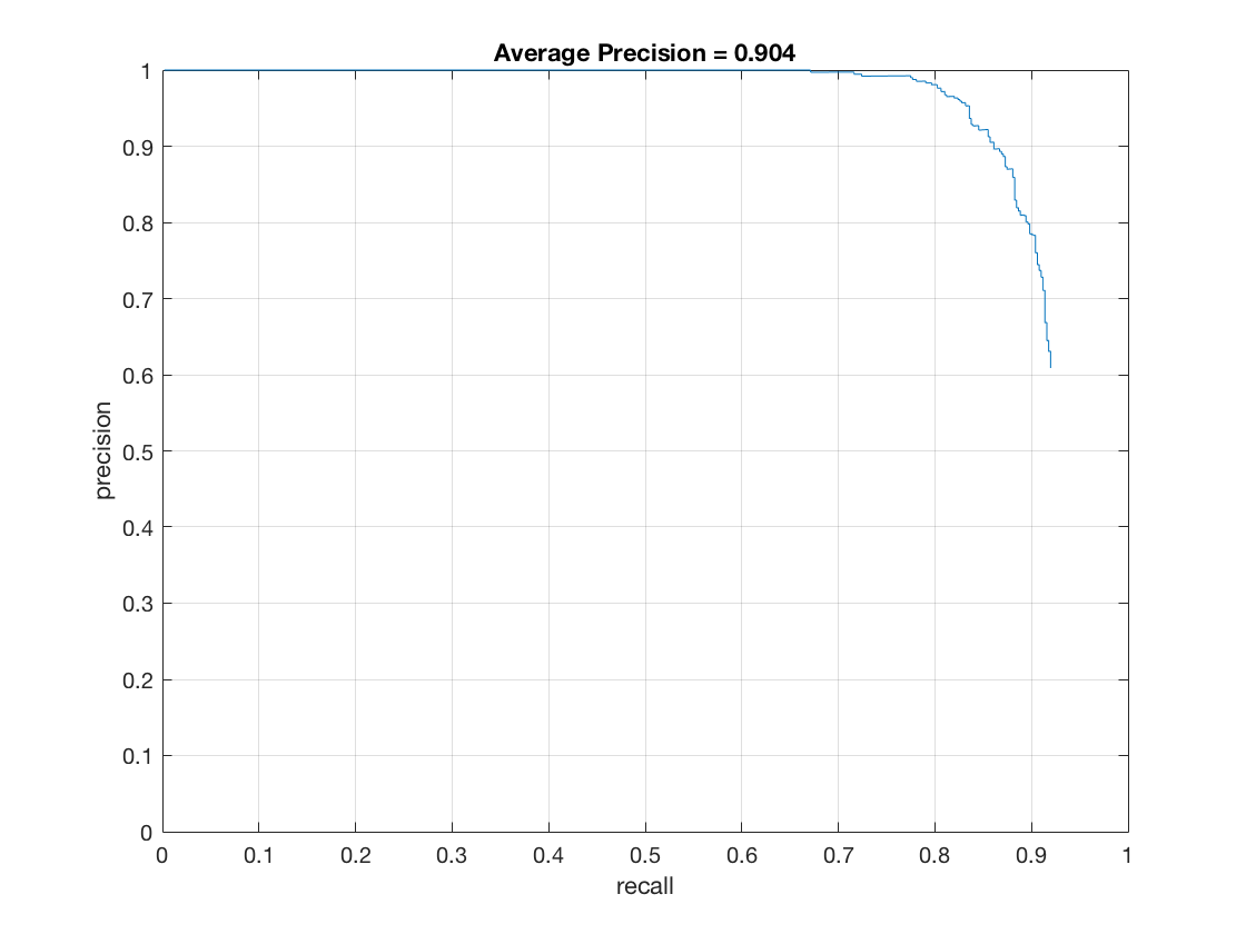
The optimal cell size was found by running multiple tests with different values. The comparision of cell sizes of 6 and 3 are detailed below. The average precision of a cell size of 3 vs 6 was .872 vs .904. Similarly, the best lambda value was obtained through testing various values (factors of 10). The size of the detector image was scaled by 90% each time for face detection. This value was determined by analyzing tradeoffs between precision and performance. Similarly, the threshold was determined by running tests. The value of 0.7 was found to be optimal. For instance, with a cell size of 6, tresholds of .65, .7, and .75 result in .863, .872, and .868 respectively. Since the random negative features are different on each run, there are slight variations in the results on each iteration. I noticed, however, that the variations weren't too significant from trial to trail.
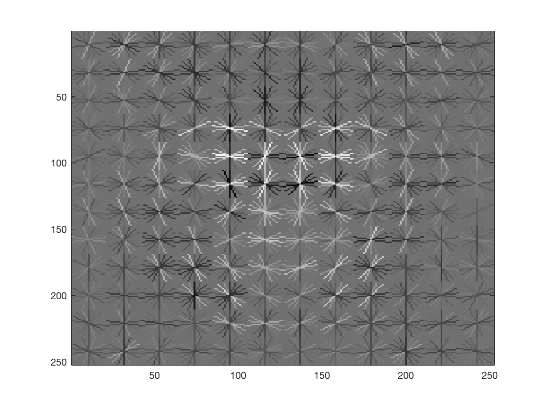
Cell size of 6 |
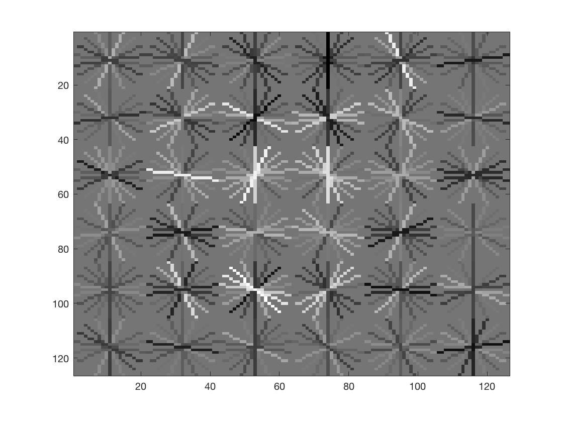
Cell size of 3 |
 Face Gradient |
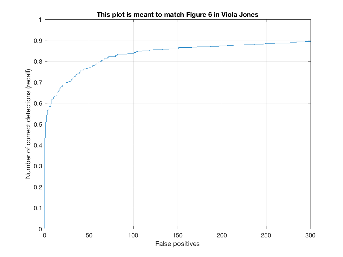 Correct v. False Positives |
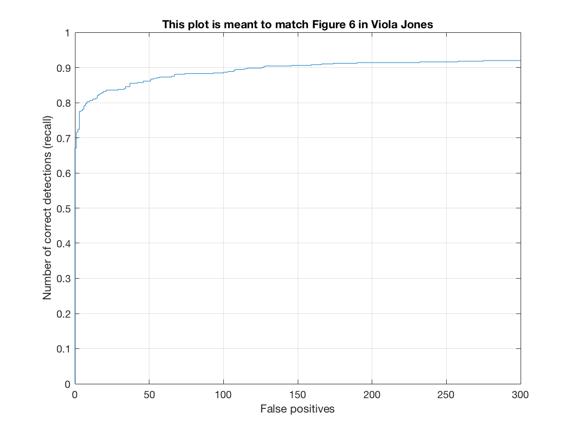 Correct v. False Positives |
 Average Precision |
 Average Precision |
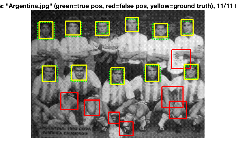 Argentina Image Sample Face Detection |
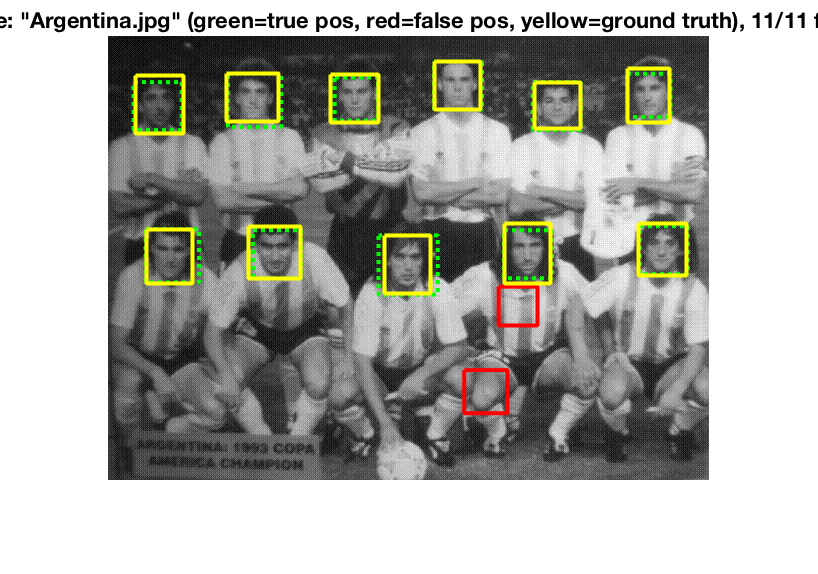 Argentina Image Sample Face Detection |
The best classifier we found was with a cell size of 3, a template size of 36, threshold of .7, scaling of .9, and a lambda of .0001. The accuracy of recognizing faces was impressively high, with a precision of ~90%. Personally, I was really amazed by the result. The process made sense, as you basically create gradients for faces and non-faces, then use a sliding window to try to find similar face gradients above a certain threshold. With larger training sets, it makes sense that accuracy would improve, as would with smaller cell sizes as more windows would be examined.
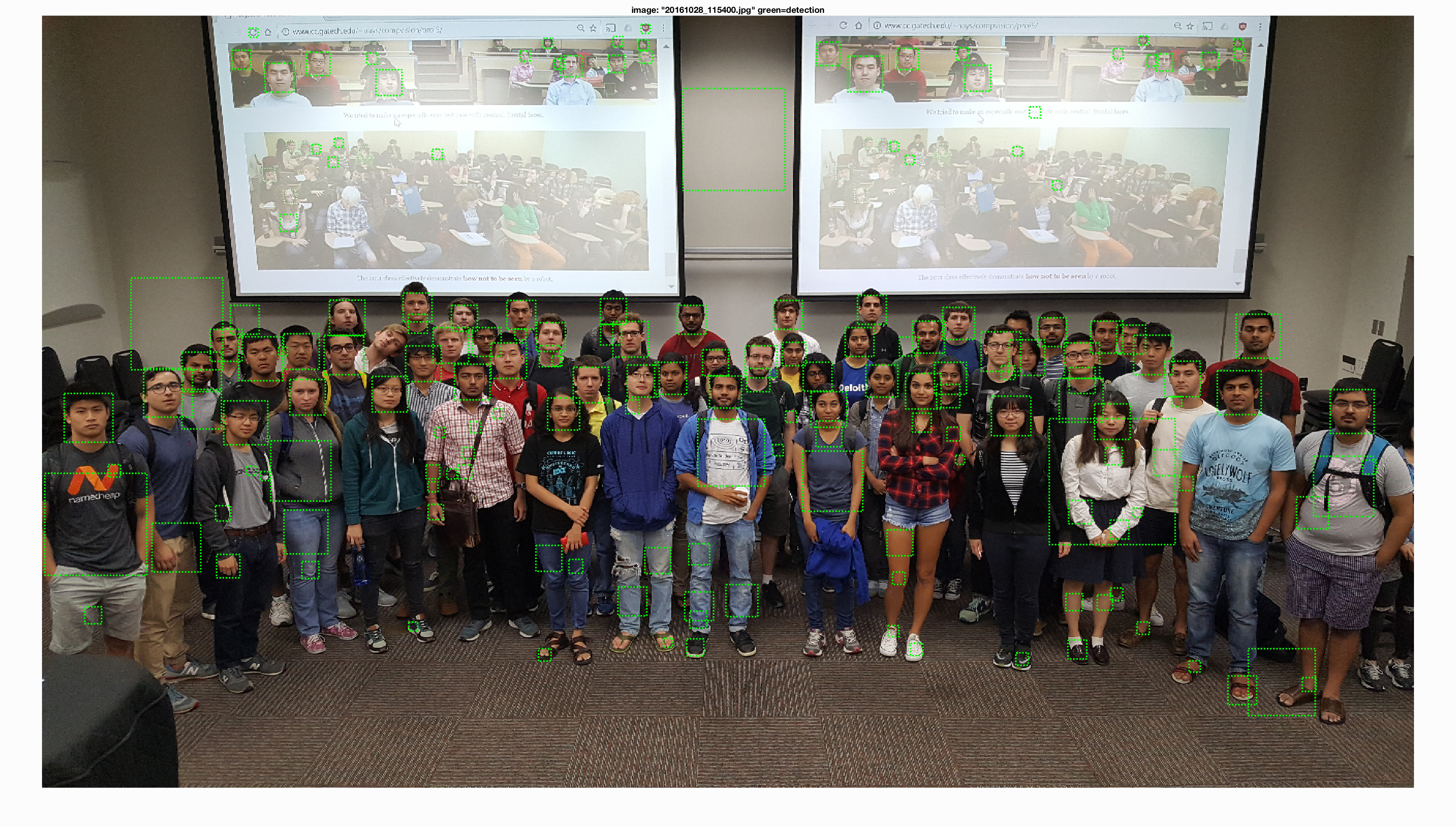 Face Detection on Class Photo |
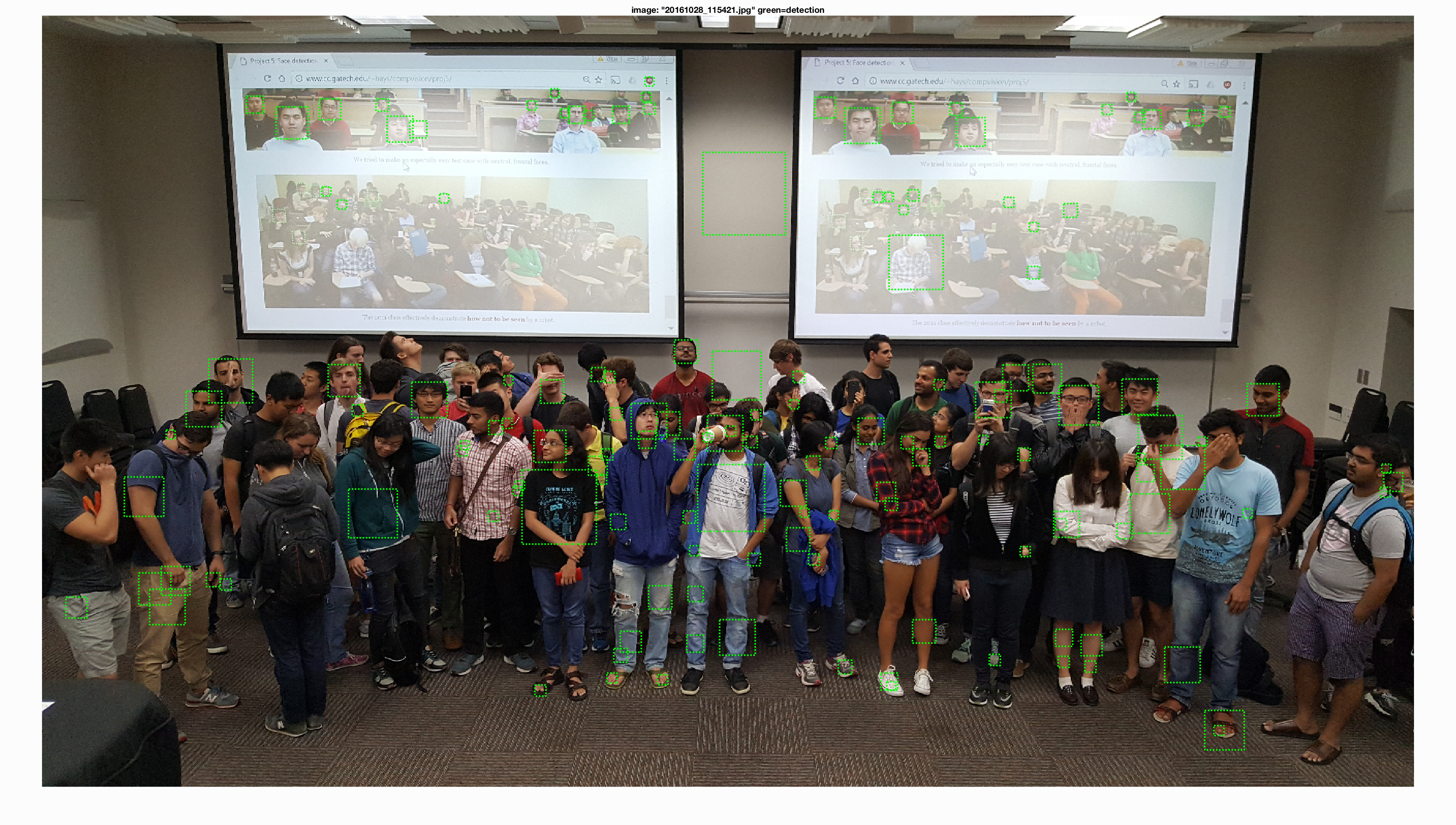 Face Detection on Difficult Class Photo |