Project 5 / Face Detection with a Sliding Window
Face detection is one of the most useful and commonly observed feature in cameras and on social networking sites. In this project, faces were detected using a sliding window approach described by Dalal and Bill .Dalal-Triggs focuses on representation more than learning and introduces the SIFT-like Histogram of Gradients (HoG) representation. Face detection was performed by training postive and negative training images and classifying using support vector maching and detecting by sliding window mechanism. The following were implemeted to identify faces in images.
- Extracting positive features
- Extracting random negative features
- Training using SVM on positive and negative features
- >Run face detector using sliding window
Extracting positive features
Positive features are training instances in which each image in the set is a 36x36 picture of a face. HOG descriptor with cell size 6 is caculates on this image. The 3d array og HOG descriptor obtained from vl_hog() is converted to 1D array. The same procedure was applied to the horizontally mirrored/flipped image to get one more HOG descriptor to increase the training data set size.
Extracting random negative features
Images in the negative training set is used to create the negative feature matrix for a given number of samples. Features are extracted from multiple scales of a single image so that the negative feature has good variation. Using the total negative samples needed samples per image is calculated. For each image number of scales sizes that can accomodate the template size is calculated as,
Training using SVM
The positive and negative features are concatenated and labels are created for them. Suppor vector machine with a lamdba of 0.0001 is used to train and w and b values are returned. vl_svmtrain comes in handy for doing the same. ( Please find the code in train_classifier.m)
Run face detector using sliding window
Thus the obtained w and b in the previous step are used to check if a part of the test image is a face or not. To find face of different sizes, image pyramid of test images are created and for each scaled image in the pyramid, HOG feature is computed. Scale value was chosen as 0.7. The number of scaled images that can be used to test for faces is computed using the above said formula. i.e. Number of scales = floor( log( template_size / image_dimension ) / log( scale_value ) ) Each window of tempate size from the computed hog cells is tested with the known w and b values. Confidence is calculated as,
Results
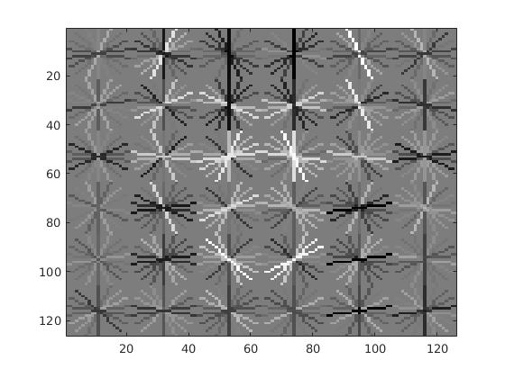
Threshold: 0.5, Lambda: 0.0001 Face template HoG visualization
Sorted by Average Precision
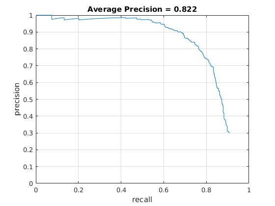
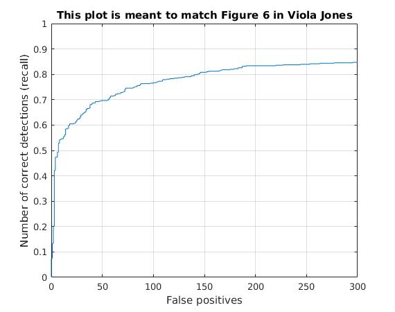
Precision Recall curve
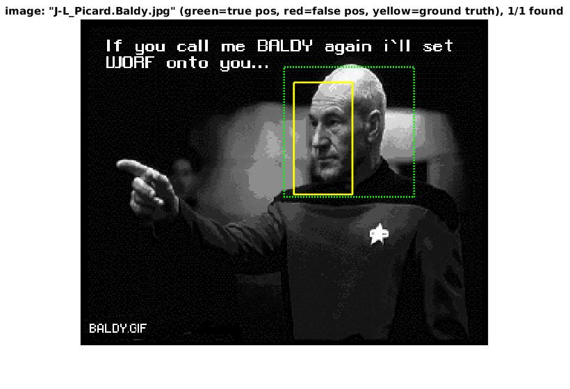
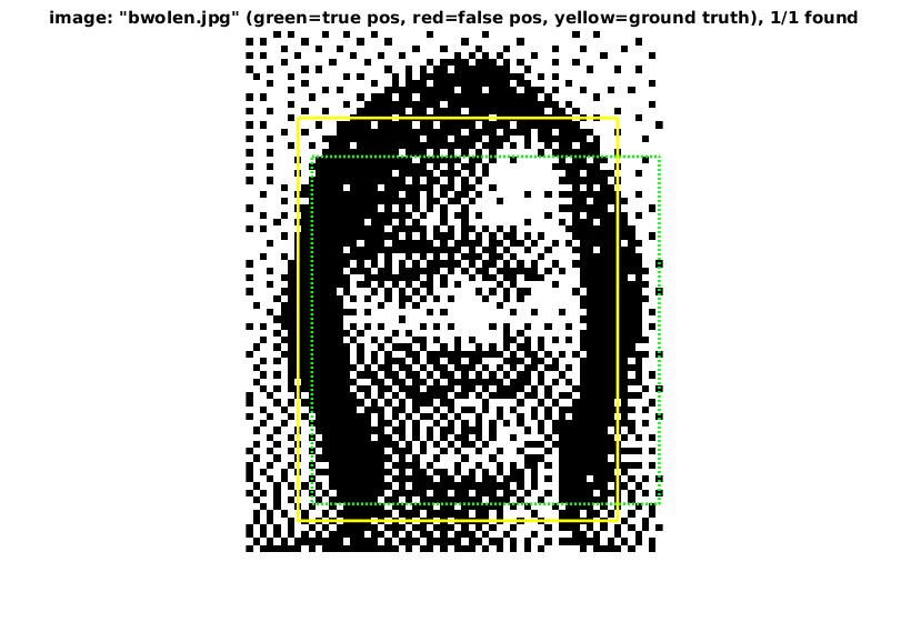
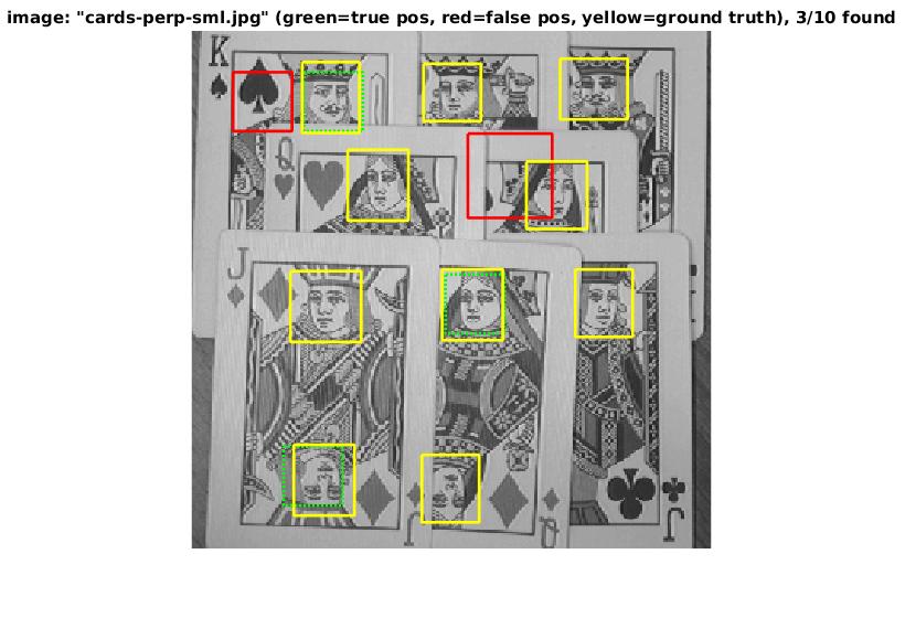
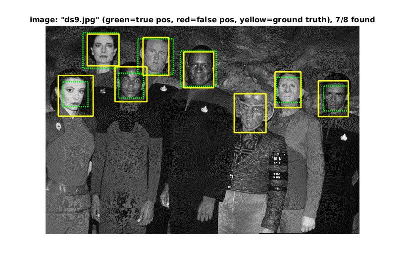
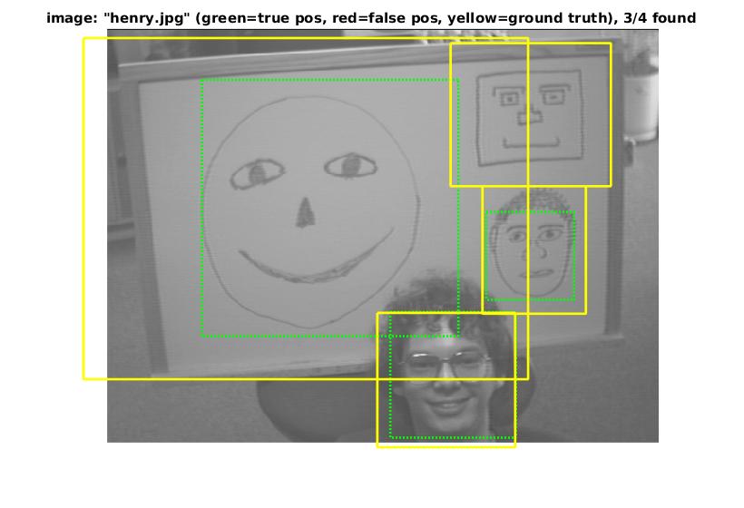
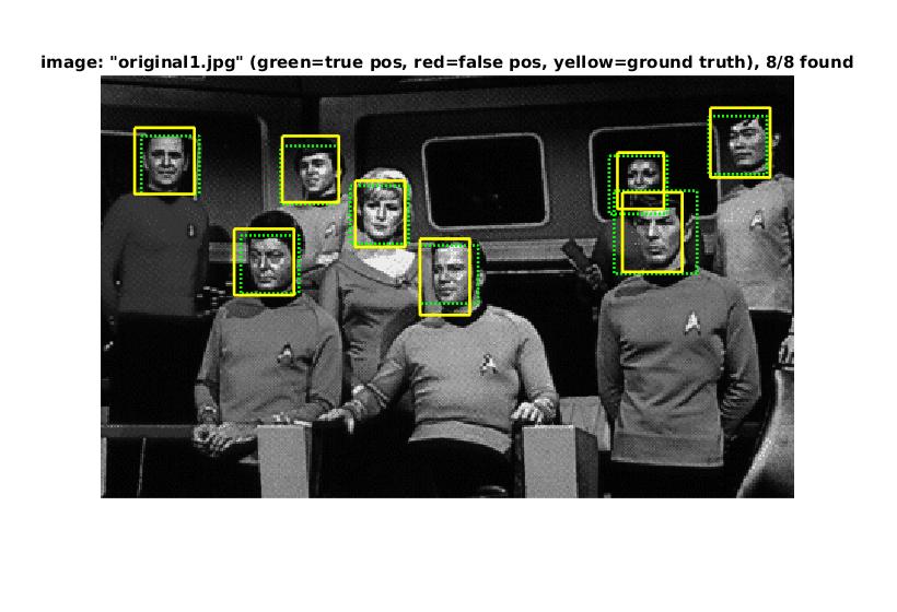
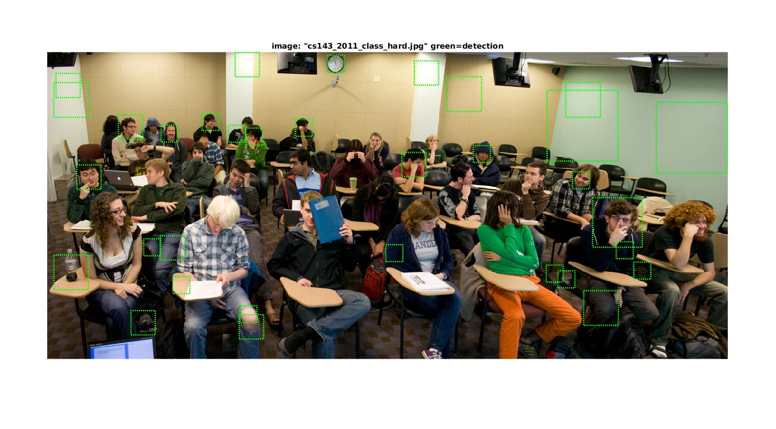
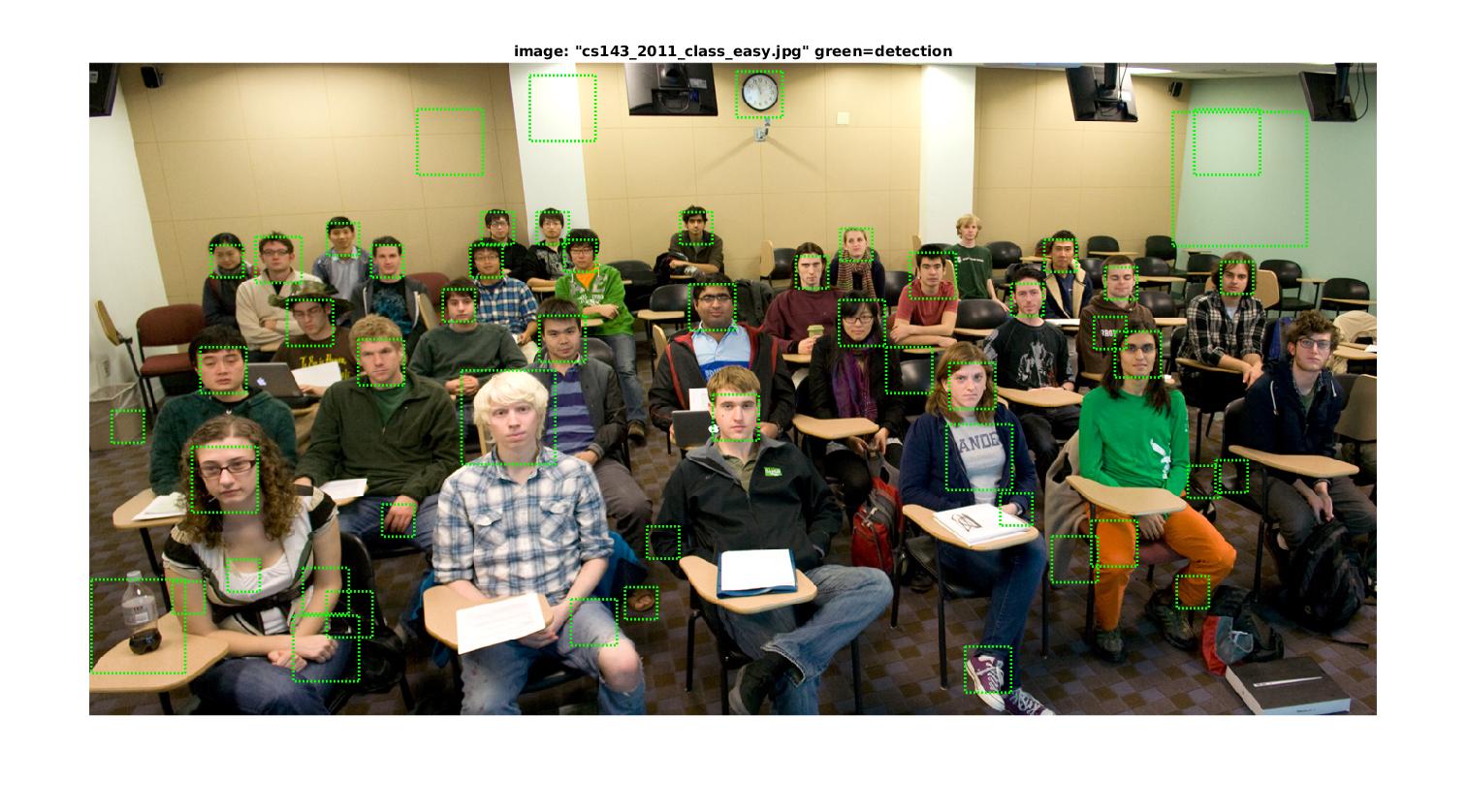
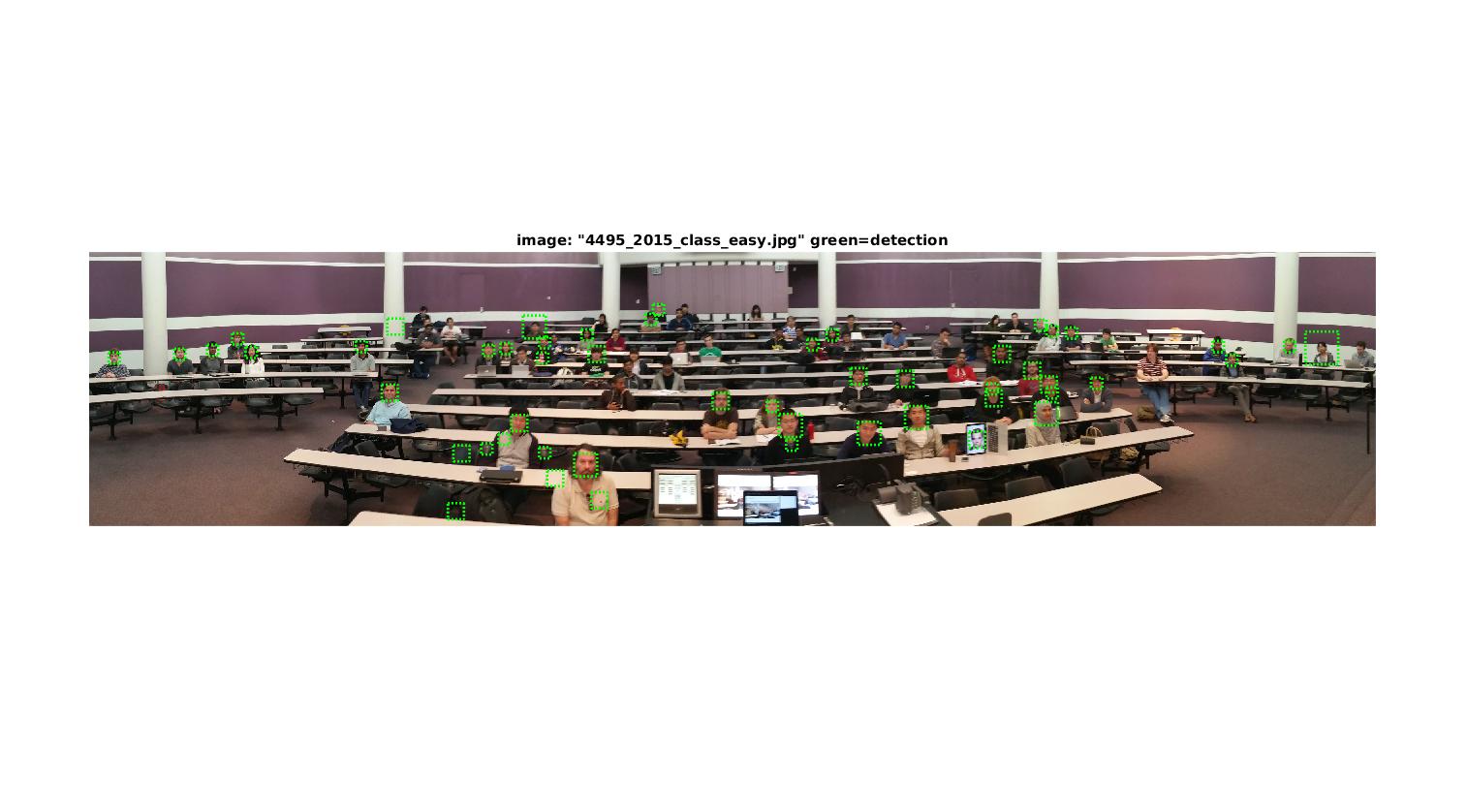
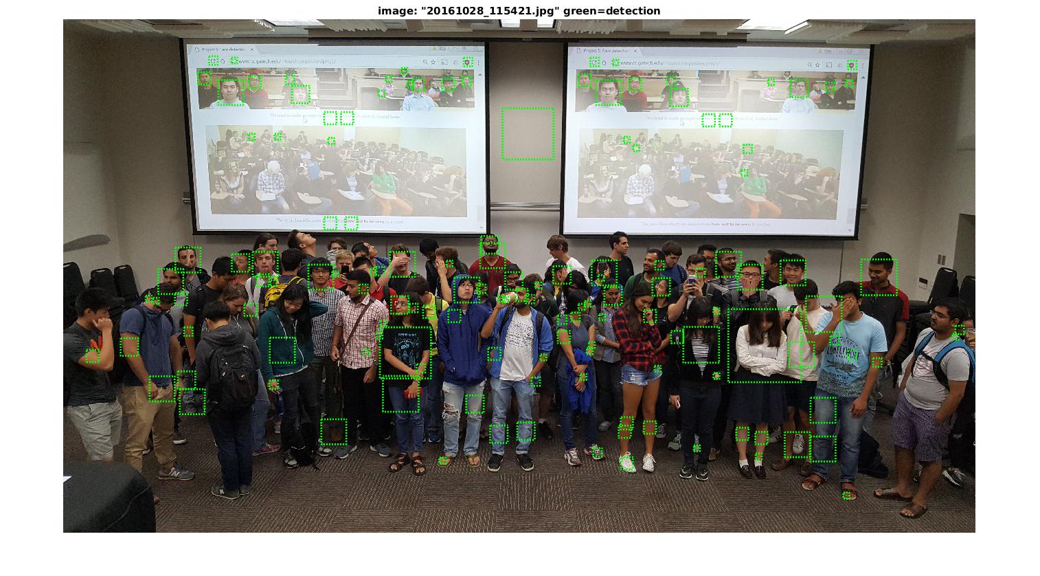
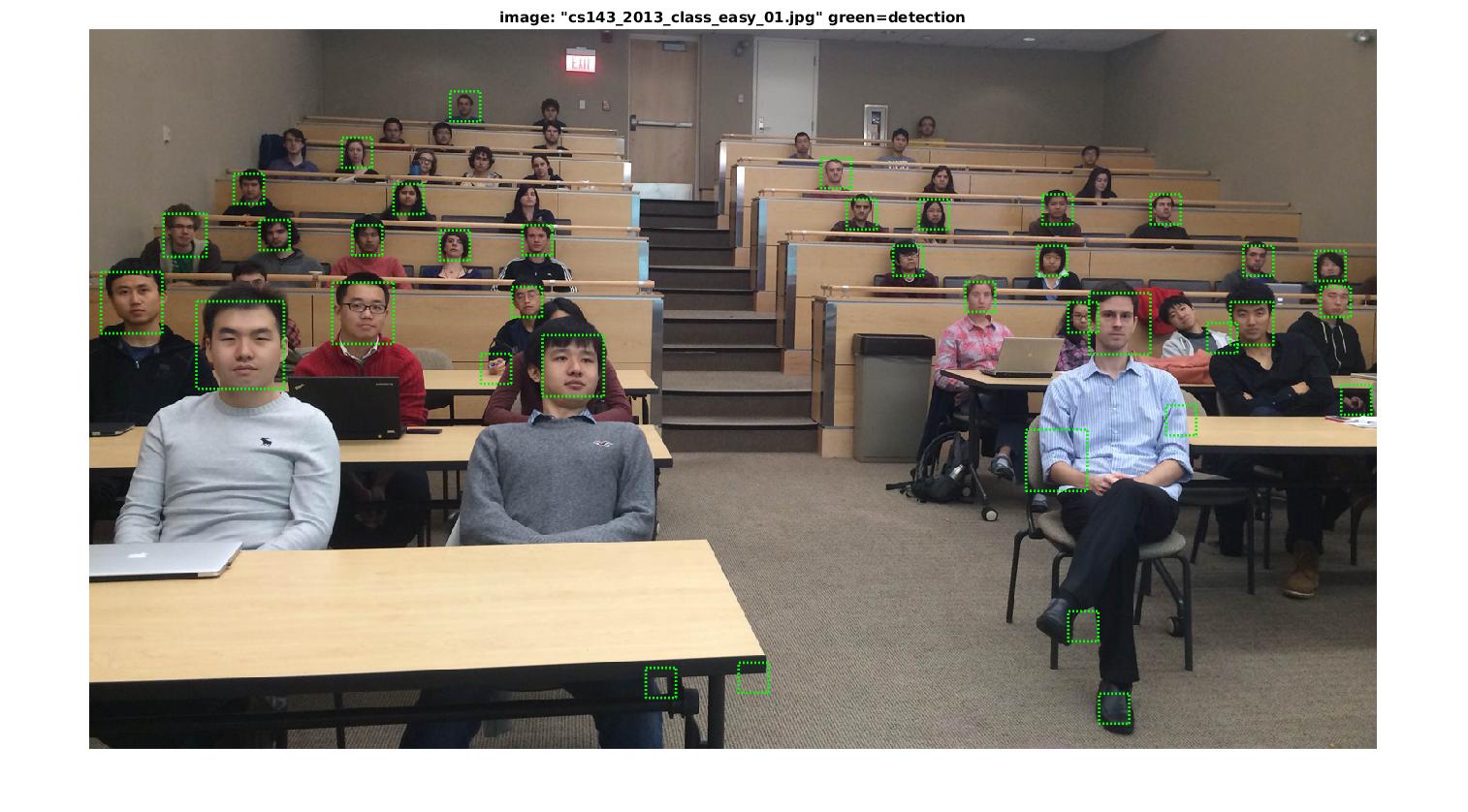
Some examples of detection on the test sets