Project 5 / Face Detection with a Sliding Window
Introduction
This report details the description implementation details, and success rates for the CS6476 face detection project. For this project, we implement a sliding window face detector using a Histogram of Gradients (HoG) feature, which was initially proposed by Dalal and Triggs. This feature is particularly well-suited to face detection, providing a high average precision in detecting faces. Initially, we build a set of features from known, positive examples and negative examples. Then, we train a linear Support Vector Machine (SVM) to learn a decision boundary between these classes. Finally, we implement a sliding-window approach to determine potential faces in an image, returning bounding boxes around all possible faces. For graduate credit, we implement a nerual network for classification and our own HoG descriptor.
Visualized SVM weights to detect face with HoG features.
Feature Selection
This section details our implementation of the feature selection process for this assignment, including the rationale behind positive and negative feature selections.
Positive Features
The first stage in the face-detection pipeline is to draw a set of a positive and negative faces. For this assignment, we have a set of approximately 6000 faces from which to
draw samples. In this case, we use all 6000 faces as positive samples. Each of these faces is pre-templated to 36x36. With the default vl__hog function, this
resulted in a feature size of (36 / cell_size)^2 * 31 . Clearly, this value changes based on the cell size. We ran three separate tests that contained cell
sizes of 6, 4, and 3 respectively.
Negative Features
Next, we retrieved negative features from a large set. Because large image can contain many possible negative feature samples, we sample randomly from this particular set. This
task is accomplished by only including those that match a sample from a distribution. That is, we only accept the sample with some probability p . For our tests, we mine
30,000 features for each run. Though a time-consuming task, this large amount of negative features allows the SVM to achieve the required success rates detailed in the
assignment.
SVM Training
This section contains details on the SVM training method. For the SVM algorithm, we utilize the given vl_svmtrain function in the vl_feat library. This SVM
learns a linear decision boundary between classes. Though only a linear classifier, we find that this particular method works fairly well in classifying faces properly. The
most important parameter for the SVM is the regularization constant. For our code, we chose a value of lambda = 0.00001 . Empirically, we found this
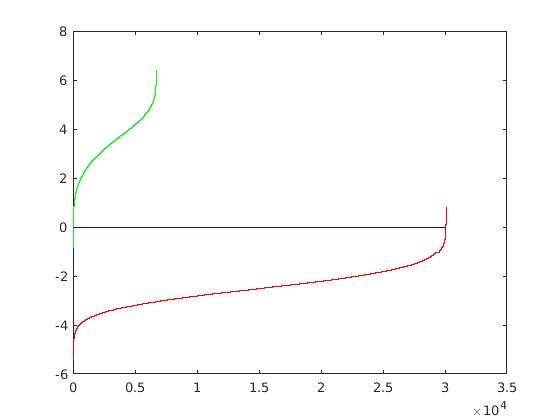
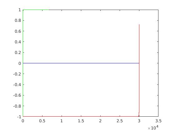
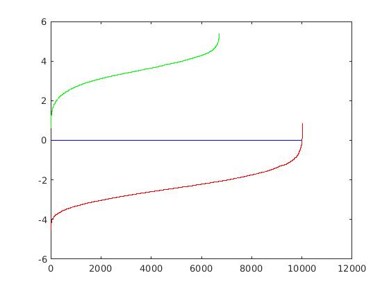
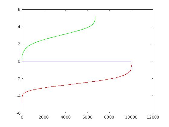
value to provide the best overall performance. The code below shows the retrieval of the parameters learned by the SVM. For each feature, a 1 corresponds to a positive
feature and a -1 corresponds to a negative feature.
	% Code showing SVM parameter retrieval
	lambda = 0.00001;
	[w, b] = vl_svmtrain([features_pos ; features_neg]', [ones(size(features_pos, 1), 1) ; ...
		-1*ones(size(features_neg, 1), 1)], lambda);
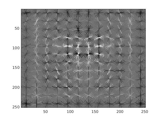
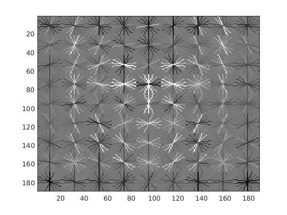
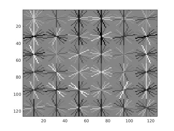
The figure below shows an example of a learned HoG descriptor face classifier. An interesting property of the classifier is that a face-like shape can be seen in the SVM weights, particularly if viewed from an angle.
|
|
Weights learned by SVM for HoG features to detect faces. An interesting phenomenon is that there appears to be an outline of a face in the weights. |
Sliding Window Approach
This section contains details on the sliding window approach taken for feature classification. For each scale selected, the window is taken as the size of the
36x36 feature template. Then, this HoG window is dragged over the image. If a particular window corresponds to a relatively high confidence, we record the
bounding box corresponding to this window. Having completed this particular scan, the next scale is given by 0.9^k where k = 0,1,2,... This
recursive approach allows for increasingly smaller window that depend on the scale of the previous iteration. This entire process is repeated for each given
test image. In this implementation, smaller cell sizes allow for smaller window steps, increasing the accuracy of the sliding-window detector.
Results
This section contains the results for the experimental runs of the classifier. In particular, in contains results for the initial required implementation. For the required graudate credit, we implement nerual networks as an additional classification mechanism and our own HoG descriptors.
Cell-Size of 6
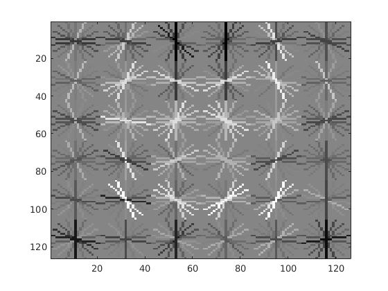
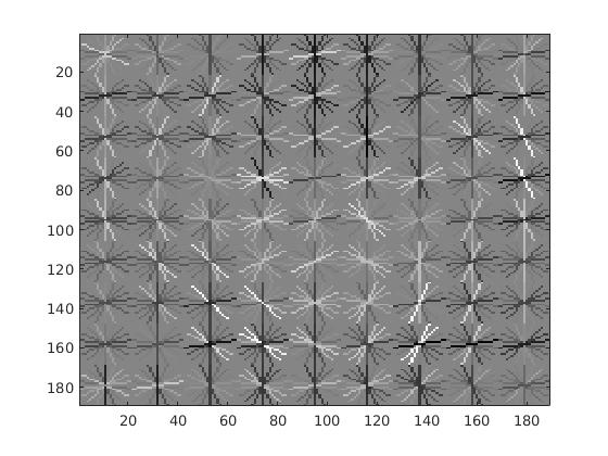
For a cell size of 6, the SVM weights and HoG visulization are displayed in the figure below.
|
|
Example weights learned by SVM and visualized HoG face detector. An interesting outcome of this process is that the visualized SVM weights look like the outline of a face. |
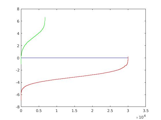
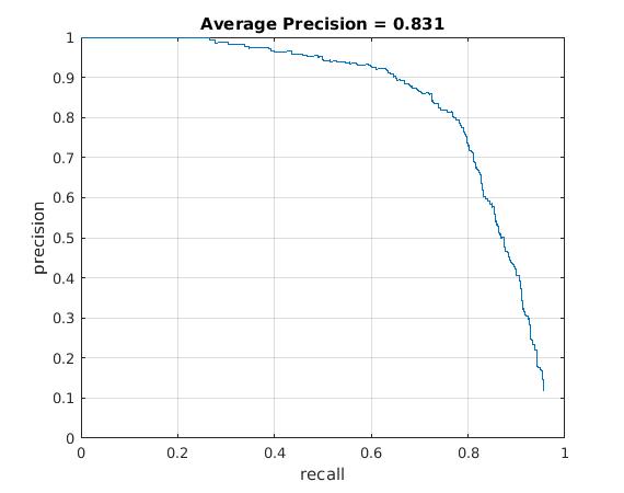
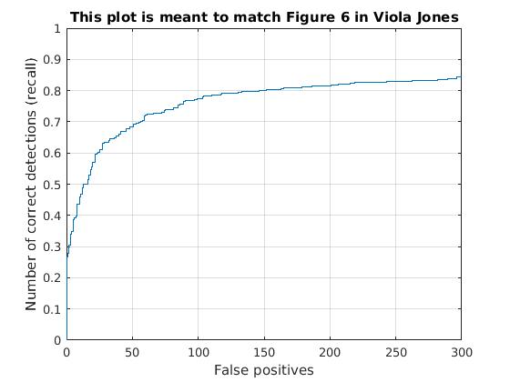
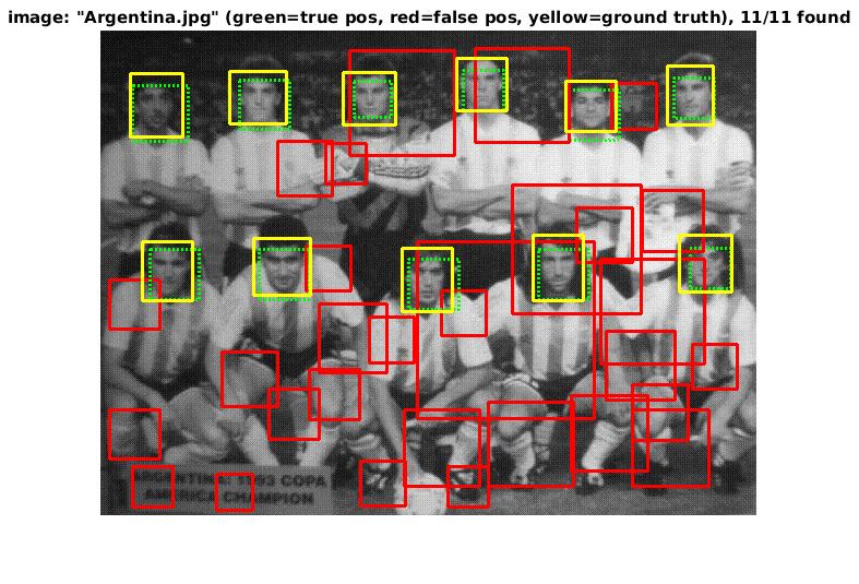
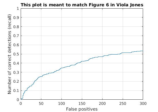
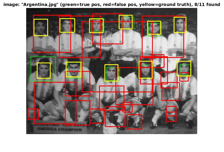
Utilizing these learned weights, the sliding window detector was run over the series of provided images. At this cell size, we achieved an average precision of 83%. The average precision and recall curve are displayed below, along with a sample image of detected faces.
|
|
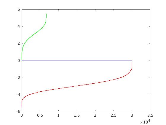
The above figure displays average precision/recall curve, recall/false positives, and a sample image of detected faces, respectively. The average precision meets the required 83%. The sample image shows detected faces. Though all faces are found, a number of false positives are also reported. |
Cell-Size of 4
For a cell size of 4, the SVM weights and HoG visulization are displayed in the figure below.
|
|
Example weights learned by SVM and visualized HoG face detector. An interesting outcome of this process is that the visualized SVM weights look like the outline of a face. |
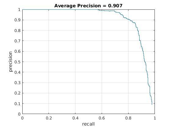
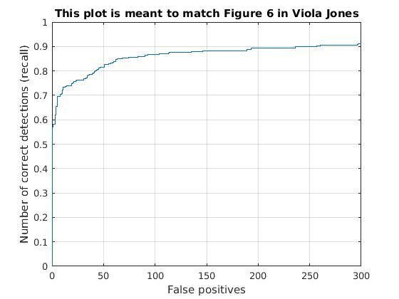
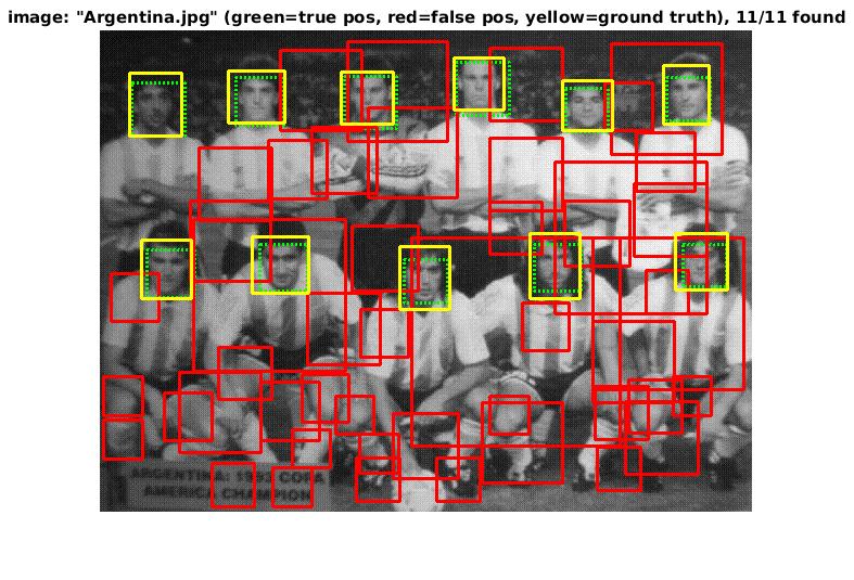
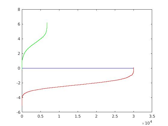
Utilizing these learned weights, the sliding window detector was run over the series of provided images. At this cell size, we achieved an average precision of 90.7%. The average precision and recall curve are displayed below, along with a sample image of detected faces.
|
|
The above figure displays average precision/recall curve, recall/false positives, and a sample image of detected faces, respectively. The average precision meets the required 89%, exceeding it to 90.7%. The sample image shows detected faces. Though all faces are found, a number of false positives are also reported. |
Cell-Size of 3
For a cell size of 3, the SVM weights and HoG visulization are displayed in the figure below.
|
|
Example weights learned by SVM and visualized HoG face detector. An interesting outcome of this process is that the visualized SVM weights look like the outline of a face. |
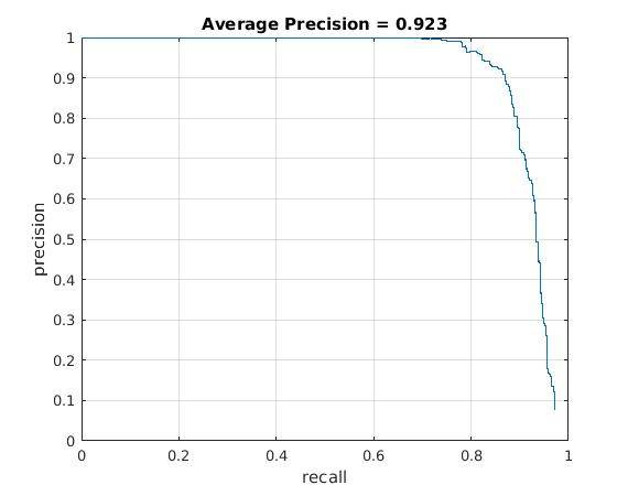
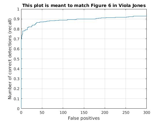
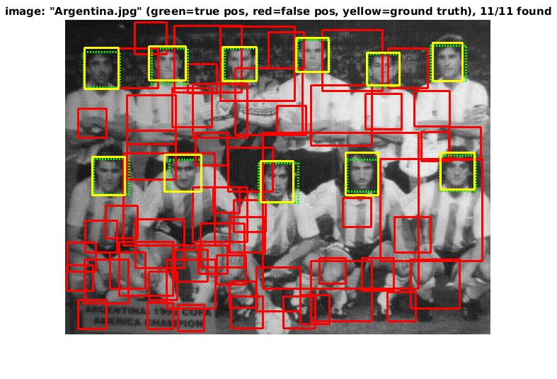
Utilizing these learned weights, the sliding window detector was run over the series of provided images. At this cell size, we achieved an average precision of 92.3%. The average precision and recall curve are displayed below, along with a sample image of detected faces.
|
|
The above figure displays average precision/recall curve, recall/false positives, and a sample image of detected faces, respectively. The average precision meets the required 92%, exceeding it to 92.3%. The sample image shows detected faces. Though all faces are found, a number of false positives are also reported. |
Neural Network Cell-Size of 6 (Grad. Credit)
For this portion, we utilized a nerual network in MATLAB with a size-12 hidden layer. For a cell size of 6, the Neural Network weights and HoG visulization are displayed in the figure below.
|
|
Example weights learned by SVM and visualized HoG face detector. An interesting outcome of this process is that the visualized SVM weights look like the outline of a face. |
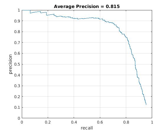
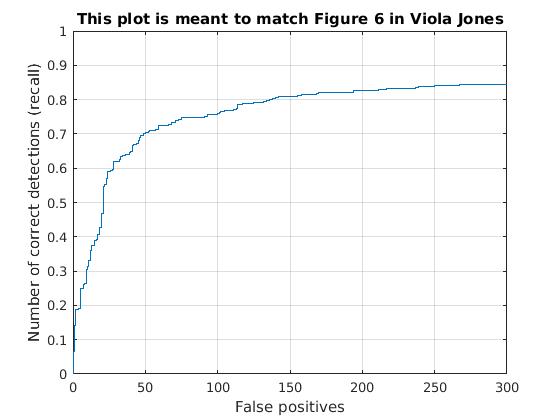
Utilizing these learned weights, the sliding window detector was run over the series of provided images. At this cell size, we achieved an average precision of 81.5%. The average precision and recall curve are displayed below, along with a sample image of detected faces. One thing to note about the nerual network classifier is that it was much slower than the SVM classifier, even though it achieved the same performance.
|
|
The above figure displays average precision/recall curve, recall/false positives, and a sample image of detected faces, respectively, for a Neural Network classifier. The average precision was 81.5%, closely matching the SVM. The sample image shows detected faces. Though all faces are found, a number of false positives are also reported. |
Neural Network Cell-Size of 4 (Grad. Credit)
For this portion, we utilized a nerual network in MATLAB with a size-12 hidden layer. For a cell size of 4, the Neural Network weights and HoG visulization are displayed in the figure below.
|
|
Example weights learned by SVM and visualized HoG face detector. An interesting outcome of this process is that the visualized SVM weights look like the outline of a face. |
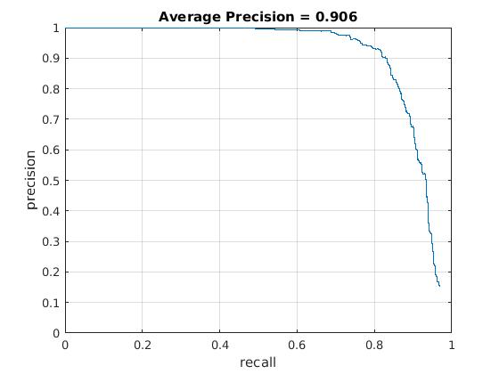
Utilizing these learned weights, the sliding window detector was run over the series of provided images. At this cell size, we achieved an average precision of 90.6%. The average precision and recall curve are displayed below, along with a sample image of detected faces. One thing to note about the nerual network classifier is that it was much slower than the SVM classifier, even though it achieved the same performance.
|
|
The above figure displays average precision/recall curve, recall/false positives, and a sample image of detected faces, respectively, for a Neural Network classifier. The average precision was 90.6%, closely matching the SVM. The sample image shows detected faces. Though all faces are found, a number of false positives are also reported. |
Implemented HoG Cell-Size of 6 (Grad. Credit)
In this section, we display the results for our implemented HoG descriptor. Overall, it was much slower than the vl_feat hog descriptor and did not provide the same average precision results. Though, the precision drop is most likely related to the usage of 10,000 negatives samples, rather than the 30,000 used in the vl_hog feature mining. For a cell size of 6, the SVM weights and HoG visulization are displayed in the figure below.
|
|
Example weights learned by SVM and visualized HoG face detector. An interesting outcome of this process is that the visualized SVM weights look like the outline of a face. |
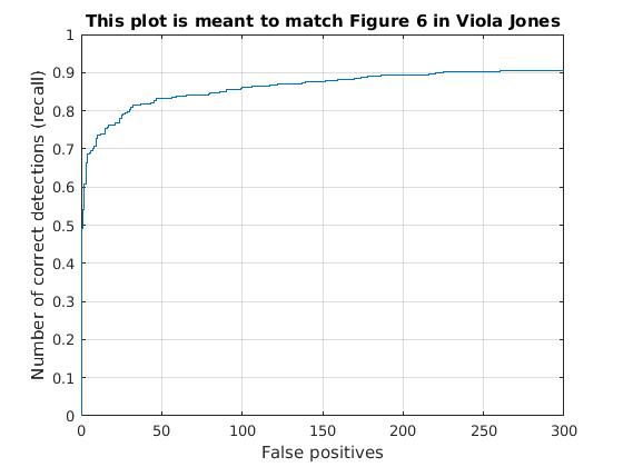
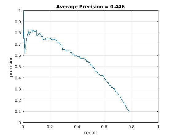
Utilizing these learned weights, the sliding window detector was run over the series of provided images. At this cell size, we achieved an average precision of 44.6%. The average precision and recall curve are displayed below, along with a sample image of detected faces.
|
|
The above figure displays average precision/recall curve, recall/false positives, and a sample image of detected faces, respectively. The average precision only reaches 44.6%, in contrast to the provided vl_feat hog features. The sample image shows detected faces. Though all faces are found, a number of false positives are also reported. |
Implemented HoG Cell-Size of 4 (Grad. Credit)
In this section, we display the results for our implemented HoG descriptor. Overall, it was much slower than the vl_feat hog descriptor and did not provide the same average precision results. Though, the precision drop is most likely related to the lack of parameter tuning within the HoG descriptor retriever function. For a cell size of 4, the SVM weights and HoG visulization are displayed in the figure below.
|
|
Example weights learned by SVM and visualized HoG face detector. An interesting outcome of this process is that the visualized SVM weights look like the outline of a face. |
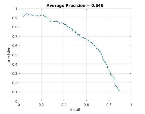
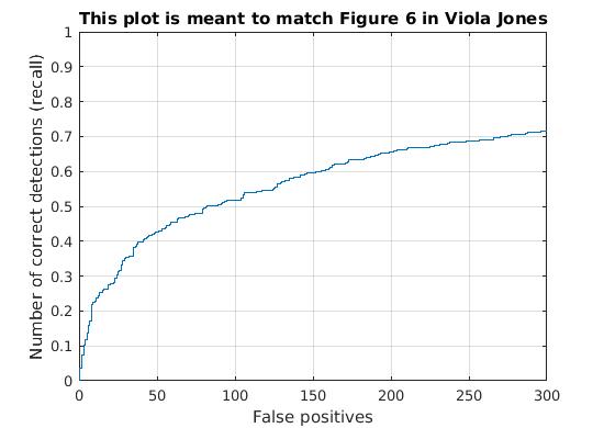
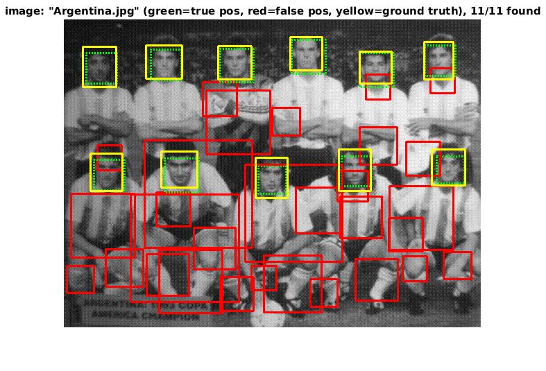
Utilizing these learned weights, the sliding window detector was run over the series of provided images. At this cell size, we achieved an average precision of 64.5%. The average precision and recall curve are displayed below, along with a sample image of detected faces.
|
|
The above figure displays average precision/recall curve, recall/false positives, and a sample image of detected faces, respectively. The average precision only reaches 64.5%, in contrast to the provided vl_feat hog features. The sample image shows detected faces. Though all faces are found, a number of false positives are also reported. |
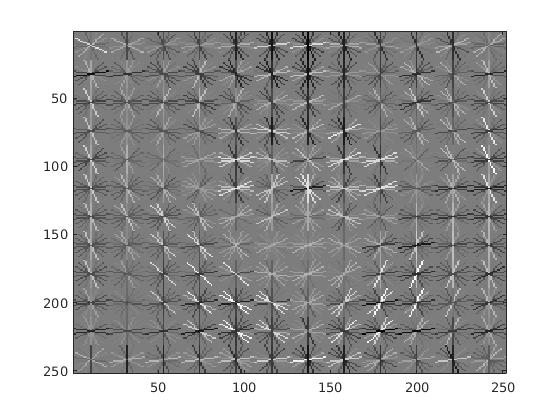
Implemented HoG Cell-Size of 3 (Grad. Credit)
In this section, we display the results for our implemented HoG descriptor. Overall, it was much slower than the vl_feat hog descriptor and did not provide the same average precision results. Though, the precision drop is most likely related to the usage of 10,000 negatives samples, rather than the 30,000 used in the vl_hog feature mining. For a cell size of 3, the SVM weights and HoG visulization are displayed in the figure below.
|
|
Example weights learned by SVM and visualized HoG face detector. An interesting outcome of this process is that the visualized SVM weights look like the outline of a face. |
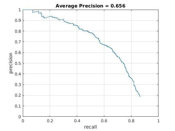
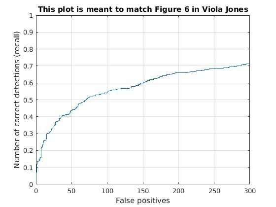
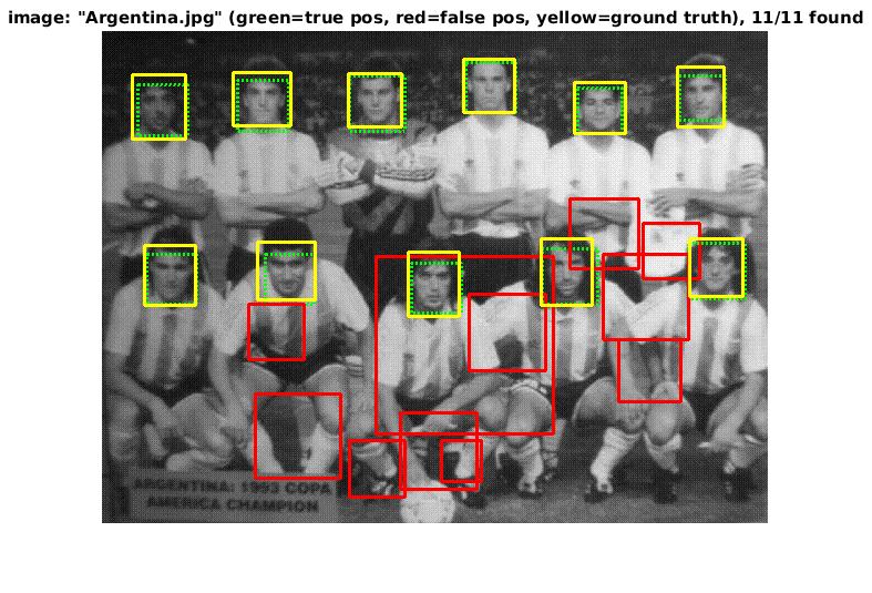
Utilizing these learned weights, the sliding window detector was run over the series of provided images. At this cell size, we achieved an average precision of 65.6%. The average precision and recall curve are displayed below, along with a sample image of detected faces.
|
|
The above figure displays average precision/recall curve, recall/false positives, and a sample image of detected faces, respectively. The average precision only reaches 65.6%, in contrast to the provided vl_feat hog features. The sample image shows detected faces. Though all faces are found, a number of false positives are also reported. |
Conclusion
In this work, we utilized a sliding window approach and SVM to detect faces in a static scene. By randomly mining negative features, using HoG features, and scaling the image repeatedly, a high average precision was obtained for this detector. The graduate credit portions for this assignment included a neural network classifier in MATLAB and an implementation of the HoG features.