Project 5: Face Detection with a Sliding Window
In this project, we will use the 'Sliding Window' paradigm, which was very popular among computer vision researchers and practitioners before the advent of deep learning. We will use this for detection of faces in an image(though given the way the problem is framed, we are really detecting heads and not faces). To do this, we will implement the famous Dalal-Triggs pipeline.
The Dalal-Triggs pipeline is simple yet gives good results. It is based on the Histogram of Oriented Gradients (HOG) descriptor operating over a sliding window of image slices in order to detect an image. Detection is performed via a classifier, in our case a Support Vector Machine (SVM). SVMs were at their peak popularity during the same time as this method. Moreover, given their quick training speed and efficient performance, they are a natural choice for a classifier.
The dataset used for training is the Caltech Web Faces project. The test benchmark is the CMU+MIT test set. The SVM and HOG implementation used is from VLFeat.
Starter Code
We run the starter code to get a baseline measure. It predicts random faces in every image and gets the following results.
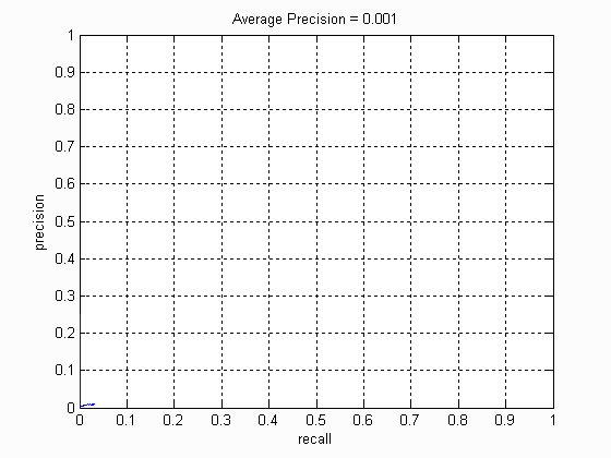
The Precision-Recall curve for this method is as follows.
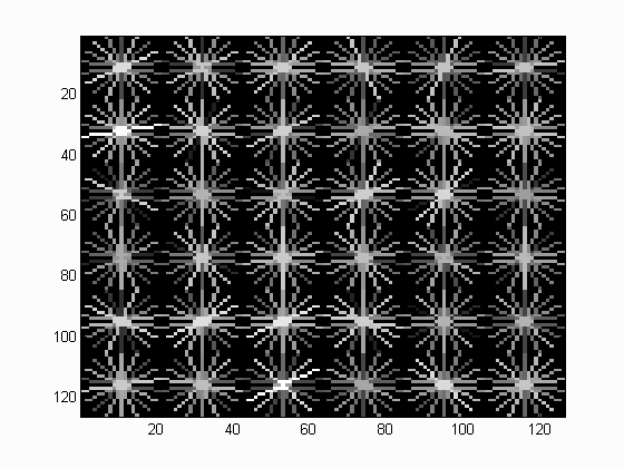
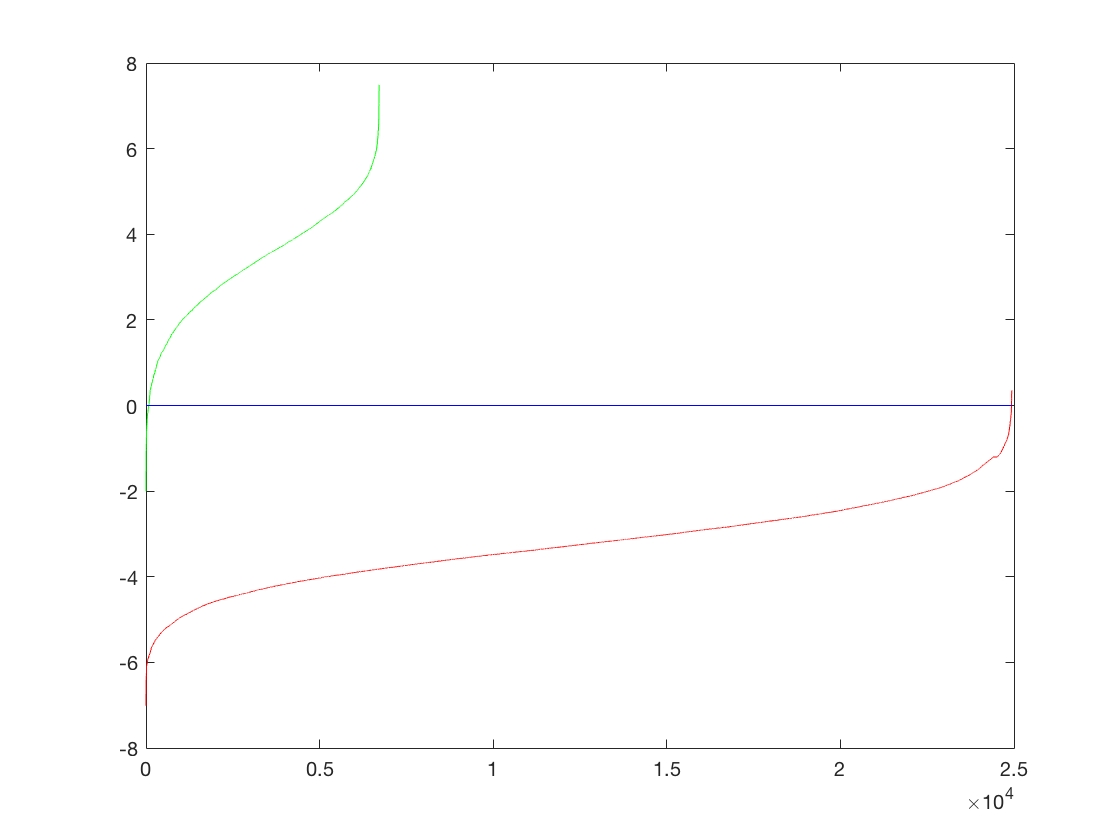
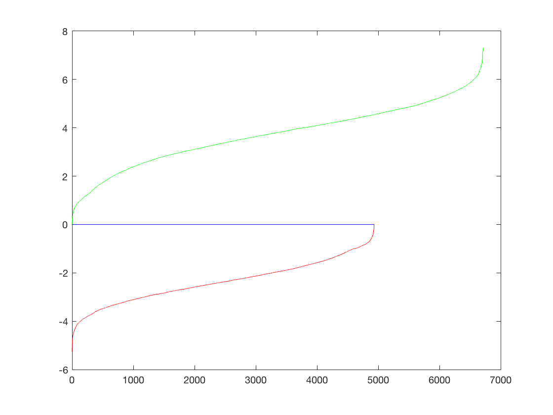
The HOG template generated by learning from the training data is as follows
See the method in action on a test image.
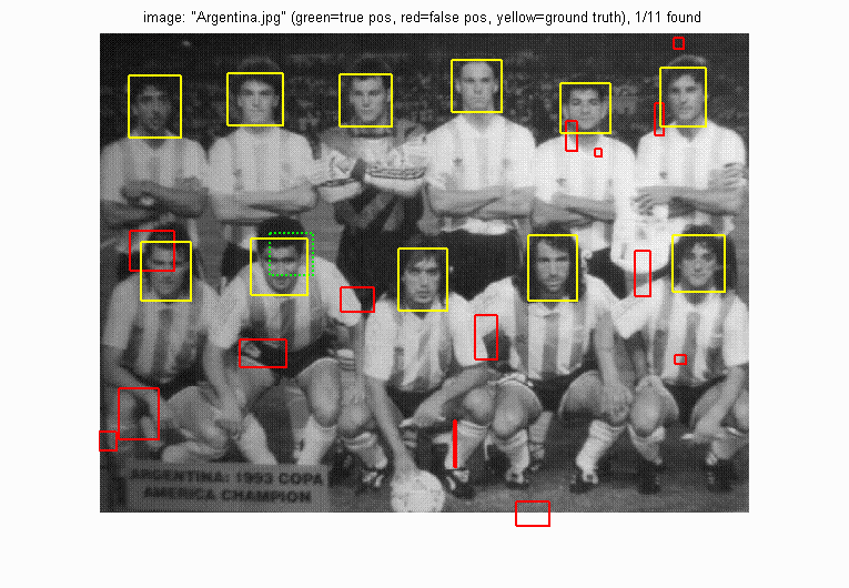
Thus, we observe that a random face predictor does not give us good precision (as expected).
Baseline Dalal Triggs Implementation
We implemented the baseline Dalal Triggs pipeline using a HOG descriptor and SVM as classifier. To ensure good classification, we sampled around ~7000 positive features and ~25000 negative features. The reason we picked a higher number of negative examples is that the feature space of faces is small as compared to the feature space of non-faces. Therefore, in order for our classifier to learn well, we must cover the non-face space adequately.
The template size was 36 and HOG cell size was 6. The performance (after tuning the parameters) is given as follows.
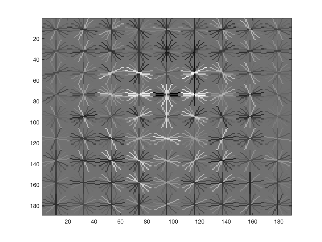
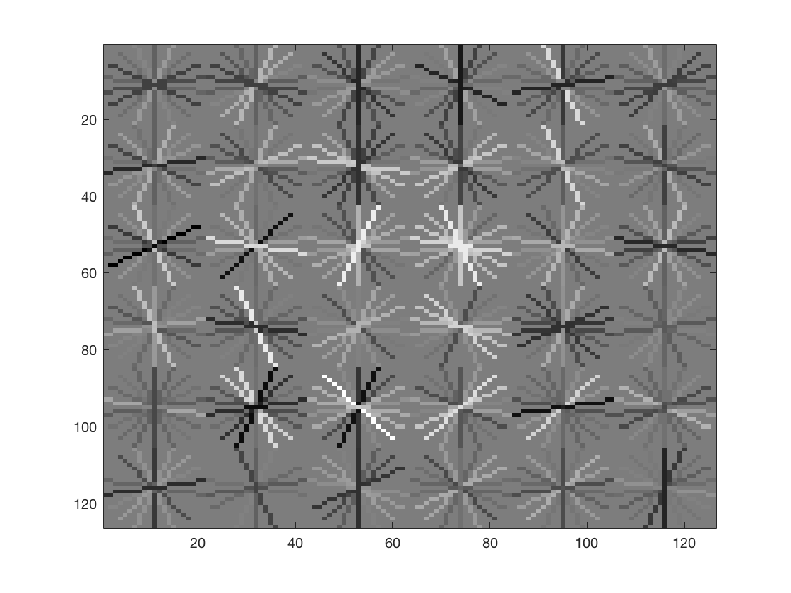
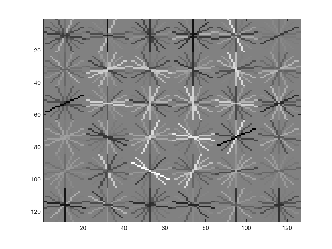
The HOG template generated by learning from the training data is as follows
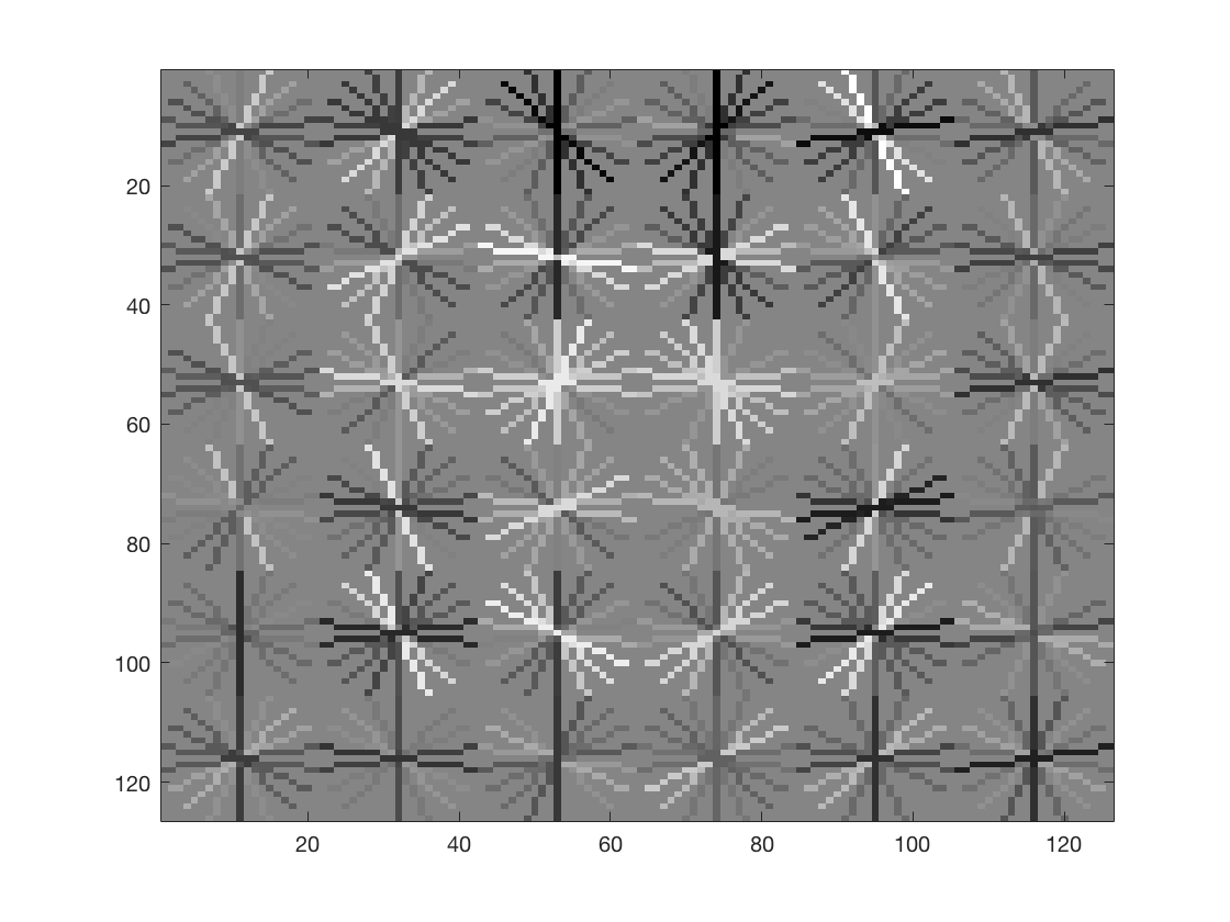
The template vaguely resembles a face like structure, which will help the classifier detect faces later in the pipeline.
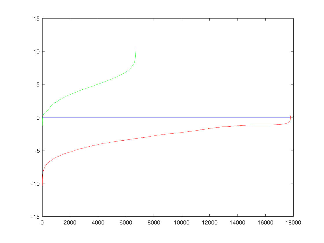
The performance on training data is as follows,
The training accuracy is 0.997 and is broken down as follows,
- true positive rate: 0.210
- false positive rate: 0.000
- true negative rate: 0.788
- false negative rate: 0.003
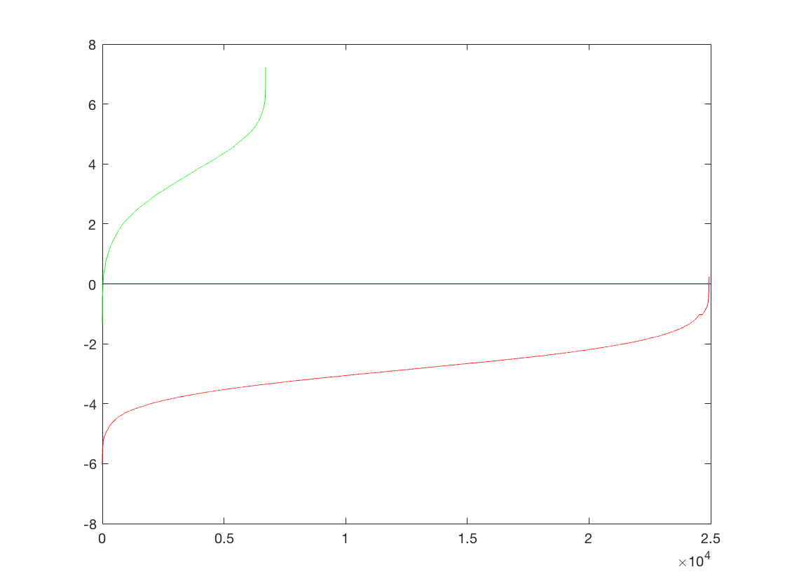
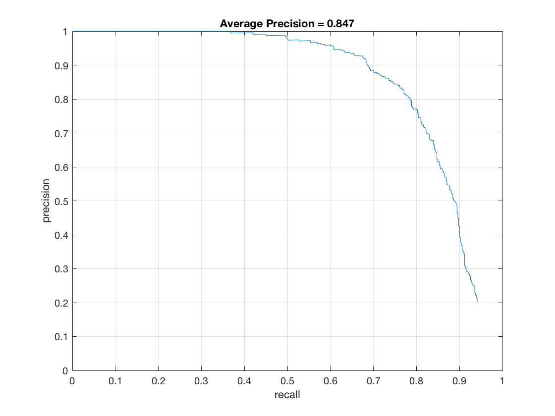
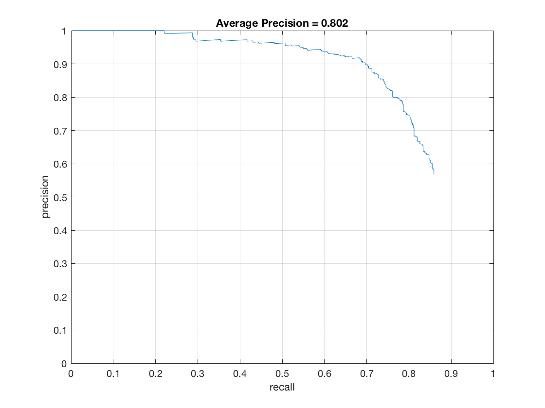
The Precision-Recall curve (on test set) for this method is as follows.
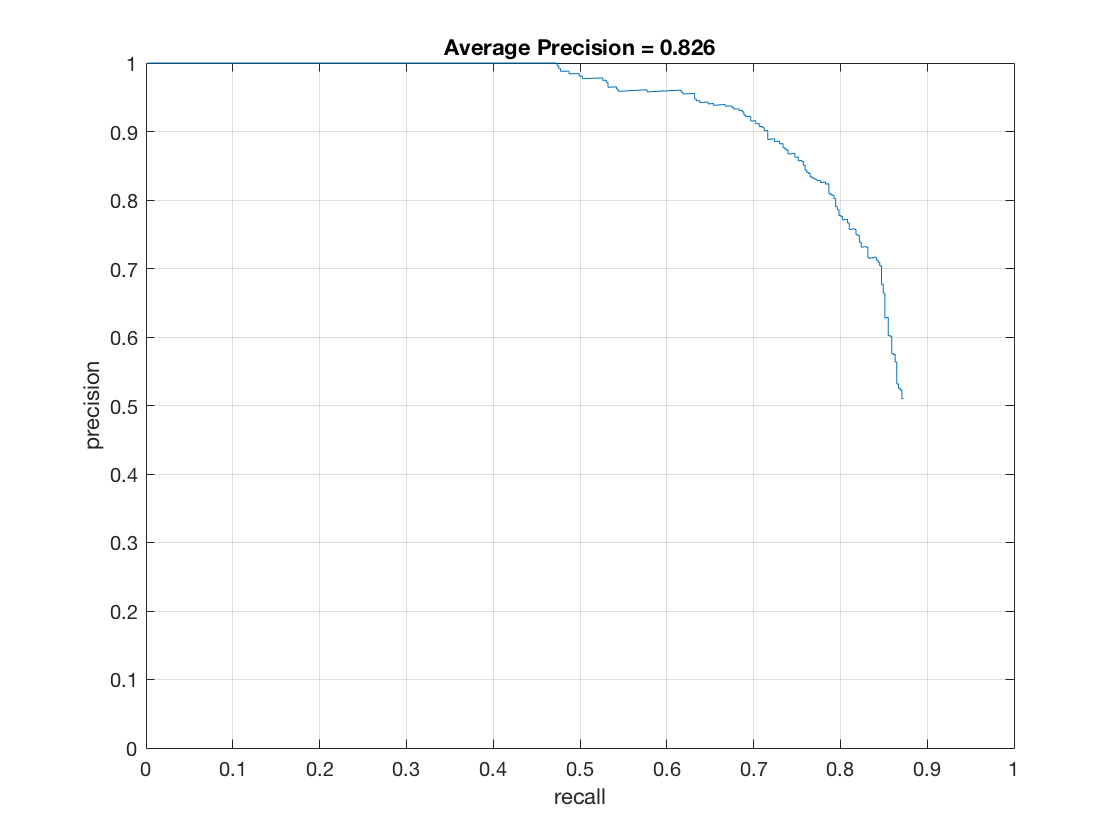
The average precision obtained is 0.826 which is expected at a step size of 6.
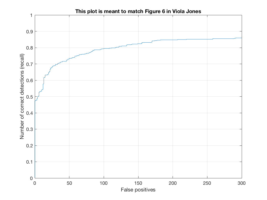
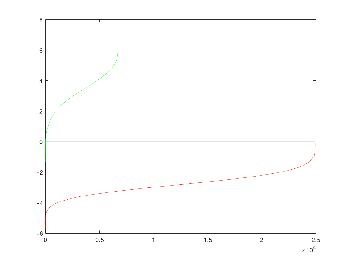
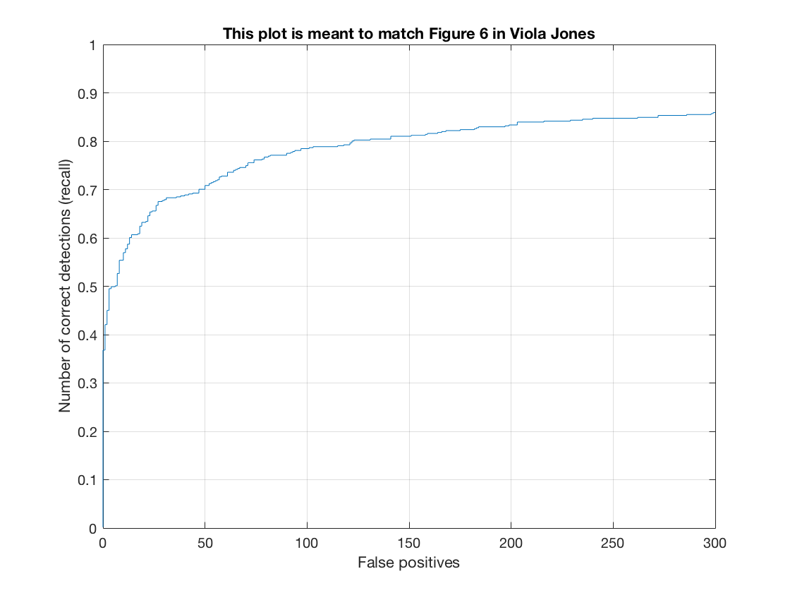
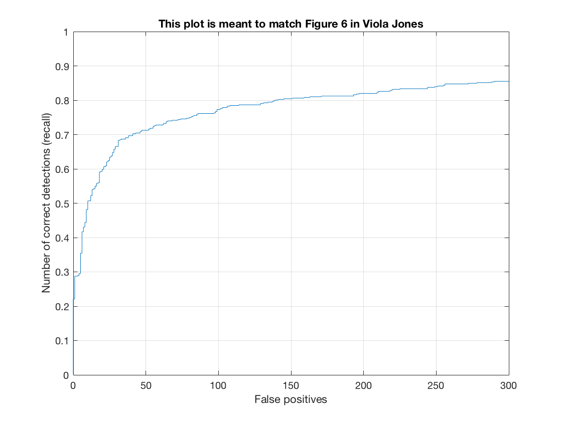
The Recall-False Positive curve (on test set) for this method is as follows.
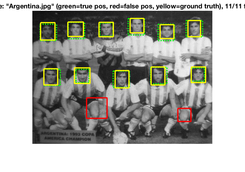
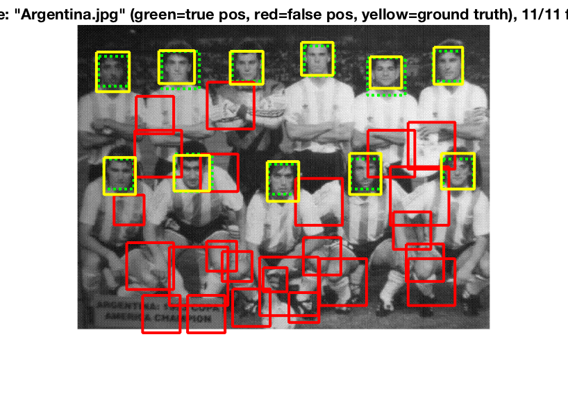
See the method in action on a test image.
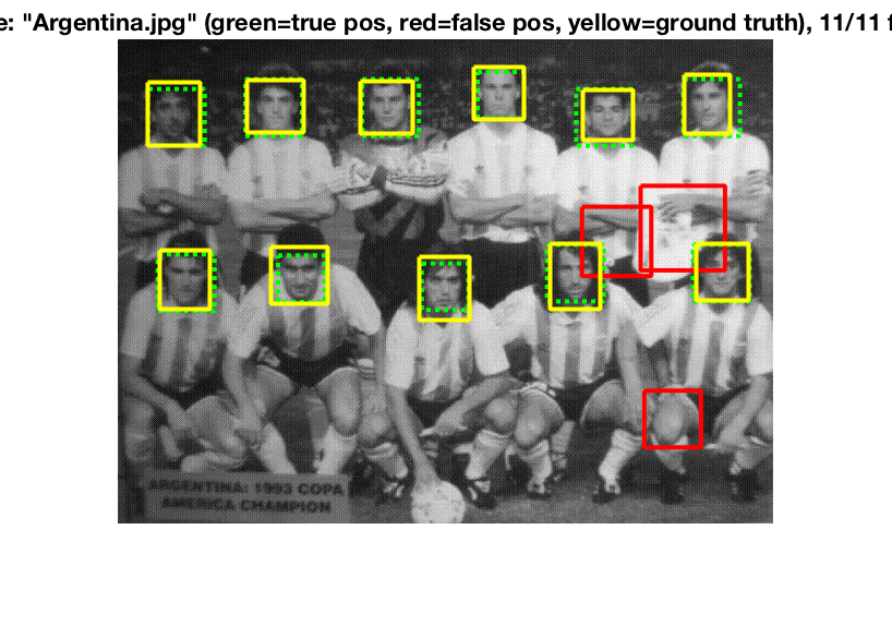
While giving us a few false positives, this pipeline gets all of the faces right in the test image.
Thus, we observe that this method gives us a much better precision as compared to our random benchmark.
Improvements on Baseline
HOG Cell Size
Now we vary the cell size of the HOG cell size and see how it affects the performance. Conventional wisdom dictates that using a finer HOG cell size should give us more details in the descriptor which would allow for better performance. However, that would come at the cost of time taken to run. We will measure this tradeoff across a HOG cell size of 3, 4 and 6.
The HOG template generated by learning from the training data is as follows (in order 6,4,3)
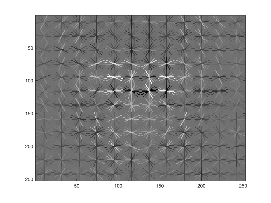
Thus we can see that a finer HOG cell size gives us a better description of a face. The third image especially, looks remarkable like a face and is much more detailed. There is a general pattern in the shape of two eyes, a nose-like bridge between them and a facial structure.
The performance on training data is as follows,
|
Cell Size |
Accuracy |
True Positive |
False Positive |
True Negative |
False Negative |
|
6 |
0.997 |
0.21 |
0.00 |
0.788 |
0.003 |
|
4 |
0.999 |
0.211 |
0.00 |
0.788 |
0.001 |
|
3 |
0.999 |
0.212 |
0.00 |
0.788 |
0.001 |
The performance is similar across the different cell sizes and does not vary much.
The Precision-Recall curve (on test set) for this method is as follows (in order 6,4,3)
|
Cell Size |
Average Precision |
|
6 |
0.826 |
|
4 |
0.883 |
|
3 |
0.911 |
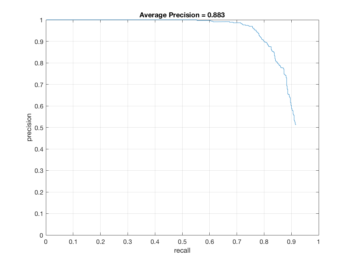
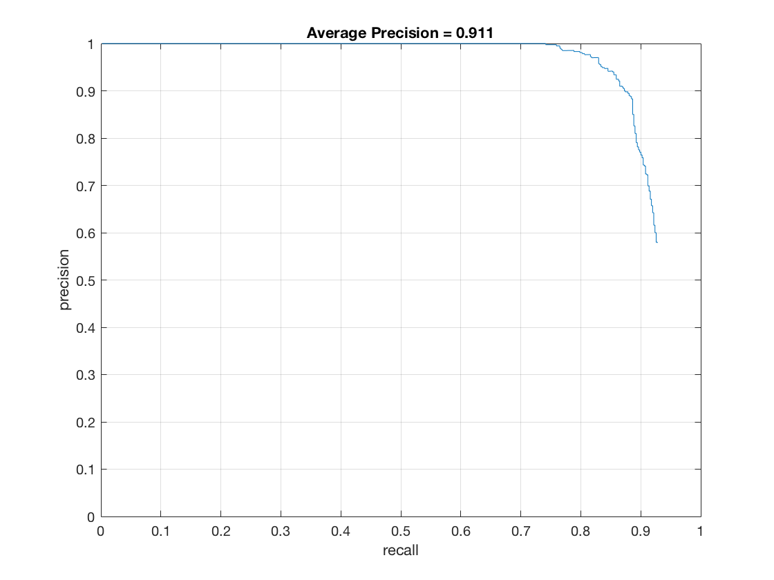
Thus, having a finer cell size leads to better and better precision. This can be attributed to the fact that the finer HOG contains more information about facial structure and better features that allow the classifier to differentiate between various images. Therefore, it is able to judge faces better.
The Recall-False Positive curve (on test set) for this method is as follows.
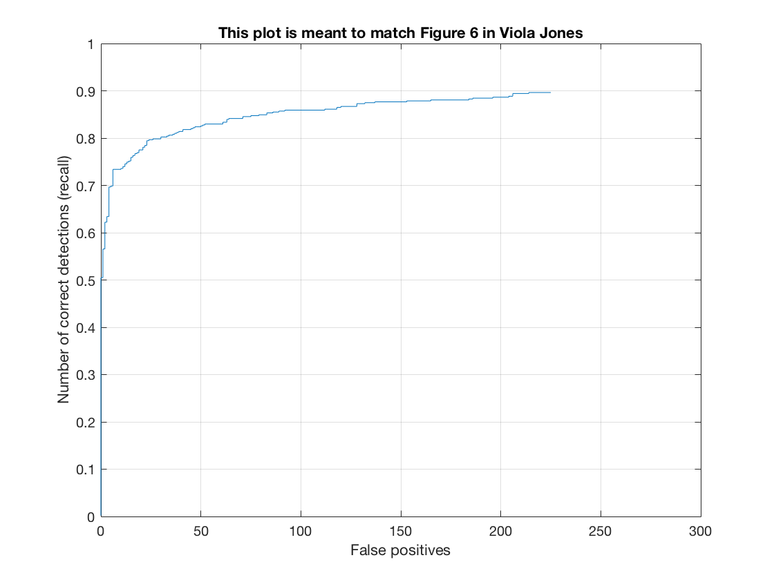
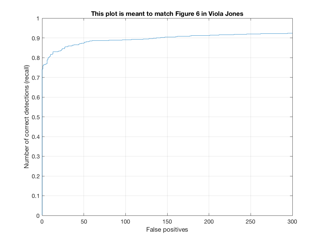
Thus, we see that as we move to a finer HOG cell size, the amount of false positives required to achieve the same level of Recall diminishes. Moreover, the point at which we must introduce false positives to get a higher recall keeps shifting upward. For example, for cell size 6, we can get a 50% recall without any false positive. For cell size 3, we can get a 75% recall without any false positive. Therefore, a finer hog cell size classifies better.
See the method in action on a test image.
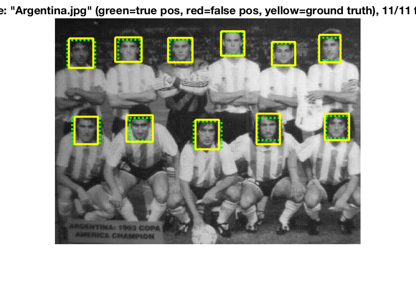
Thus we see what we have learned from the above charts in action. Each time all faces in the picture are detected, however, the finer the step size, the lower the number of false positives.
The time taken by each method is as follows
|
Cell Size |
Feature Sampling (s) |
Training (s) |
Detection (s) |
|
6 |
16.751657 |
0.578759 |
31.440676 |
|
4 |
18.370874 |
1.936797 |
56.195079 |
|
3 |
20.977181 |
5.582813 |
133.560870 |
Thus, we see that having a finer HOG cell size gives us a better descriptor, which helps the classifier better understand the space and ultimately achieve a higher level of precision in detecting faces. However, the tradeoff is in terms of time. While having a finer cell size does lead to increases in time required for feature sampling and training the classifier, the major chunk of the pipeline is in detection and the speed of the detector is inversely proportional to the fineness of the HOG cell. Therefore, a finer HOG cell size gives us higher precision at the expense of more computation.
Class Photos
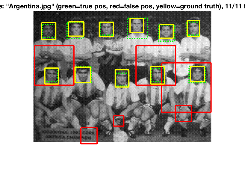
We tried out the best performing classifier on the class photos and got the following results.
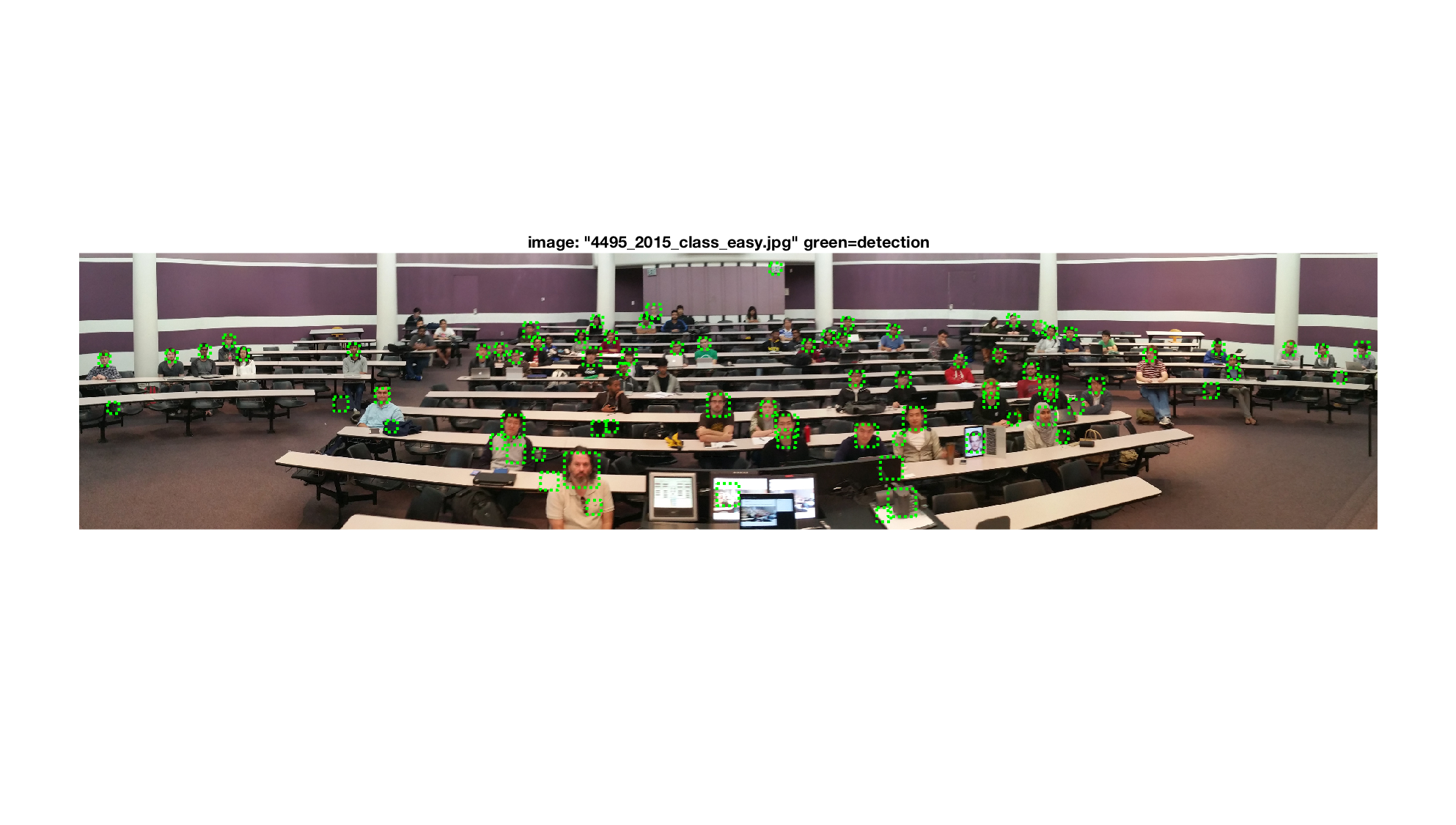
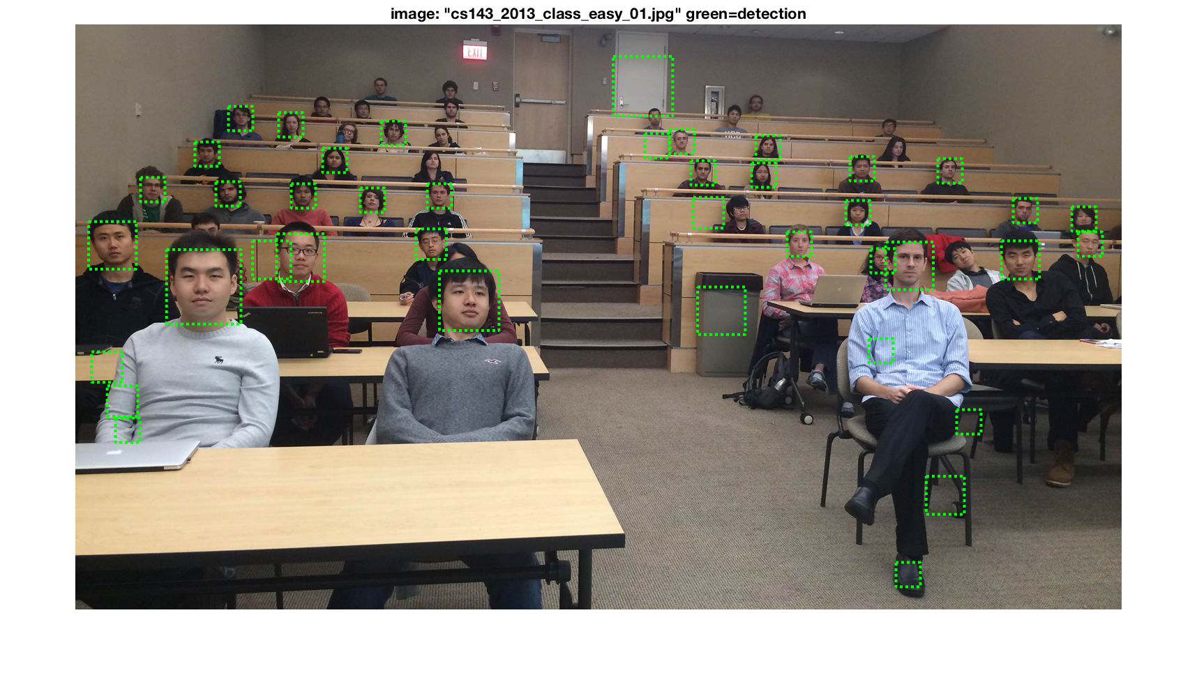
We observe that the classifier detects faces in the easy pictures, with some false positives.
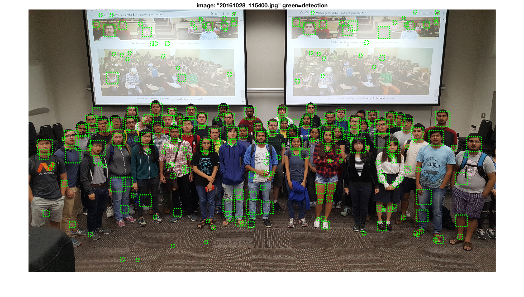
In the above picture, we can see that the classifier detects many faces (including the ones in the picture projected on the screen), however there are some false positives as well.
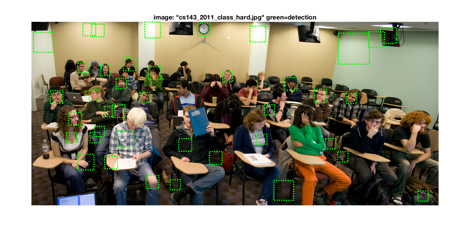
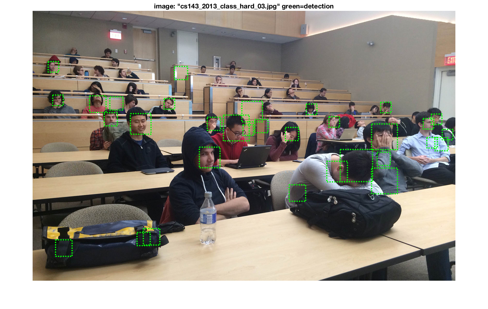
On the hard images, we can see that the classifier is unable to detect some faces however, due to obfuscation, it seems to miss many facial structures in the image.
Our classifier is built to prefer a higher recall at the expense of false positives (becuase they're essentially ignored if the confidence is low enough). Therefore, to arrest the high number of false positives, we will make a variant.
Hard Negative Mining
Hard Negative Mining is an iterative method of improving the accuracy of the classifier. We take the false positives obtained in one pass and retrain the classifier on them, labelling them as negative training input. This helps the classifier better distinguish the images the next time around.
This technique is useful when the number of negative training examples is limited. In our case, we have sampled for a lot of negative training examples, therefore we cannot see the effects of hard negative mining. Therefore, to see the effects, we must first artificially constrain our classifier with a few negative training examples and then apply hard negative mining to see the difference. We use a HOG cell size of 6. We artificially constrain our negative examples to about ~5000. We have around ~6000 positive features.
Constrained Classifier
Here, we will showcase the performance of the constrained classifier.
The HOG template generated by learning from the training data is as follows
This looks like a decent descriptor of a face.
The performance on training data is as follows,
The training accuracy is 1.000 and is broken down as follows,
- true positive rate: 0.576
- false positive rate: 0.000
- true negative rate: 0.423
- false negative rate: 0.000
The Precision-Recall curve for this method is as follows.
Thus we see that we are able to get a pretty good precision using this classifier. It even exceeds the precision of the classifier we trained on randomly sampled negative data.
The Recall-False Positive curve (on test set) for this method is as follows.
See the method in action on a test image.
Comparing this to our original classifer, we see
It is over here that we see the failing of not having enough negative examples. We can see that there are a high number of false positives for our image, even though it detects all the faces in the image.
Thus, we need to fix the problem of high false positives. Therefore, we train our classifier on randomly picked false positive results, labelling them as negative training data instead.
Constrained Classifier + Hard Negative Mining
Here, we will showcase the benefits of Hard Negative Mining.
We mined around ~12500 randomly picked false positive samples. Thus, the total number of negative samples was around ~17500.
The HOG template generated by learning from the training data is as follows
This looks like a good descriptor of a face.
The performance on training data is as follows,
The training accuracy is 0.999 and is broken down as follows,
- true positive rate: 0.273
- false positive rate: 0.000
- true negative rate: 0.726
- false negative rate: 0.001
The Precision-Recall curve for this method is as follows.
Thus we see that we are able to get a pretty good precision using this classifier. It is a little less than the precision we got earlier however.
The Recall-False Positive curve (on test set) for this method is as follows.
See the method in action on a test image.
Thus, we see here that even though our classifier gives us a small decrease in precision, it gives us less false positives. Thus, we demonstrate the effects of hard negative mining.
Parameter Tuning
Parameter tuning was necessary in order to optimize the pipeline at every step. Some useful hints were given in the starter code (like the value of lambda=0.0001 for SVM) and just required verification while others required experimentation.
Scaling Factor and Number of Scales
We performed scaling recursively, by taking consecutive powers of the scaling factor. Some of the images had a high resolution and required significant downscaling before the faces could fit inside our template sized bounding box.
A lower scaling factor downsamples aggressively. Therefore, the number of times scaling is required is less which makes execution faster. A higher scaling factor has a more fine downsampling, which requires higher number of iterations of scaling. However, it gives us the benefit of having a greater probability of catching an image that would have been missed otherwise. This is becuase it down samples more slowly and thus can capture images of various sizes. Taking these considerations into mind, we found that a scaling factor of around 0.8-0.84 worked well.
Threshold
The threshold determines the precision recall rate as it controls what images are labelled true. We used the confidence generated by the SVM as a threshold. Having too low of a threshold results in a lot of false positives while having a high threshold impacts precision. We tuned this parameter for every case separately. Typical values of threshold were in the 0.4-0.5 range. However, for hard negative mining, we found that decreasing the threshold gave us better results.
Lambda
As mentioned above, the value of lambda given in the comments was helpful and turned out to be the optimal value of lambda. This was verified by experimental results. However, after hard negative mining, we had to tune lamda.
Resources
Project 5 DescriptionDalal Triggs
Caltech Web Faces
CMU+MIT Dataset
VLFeat
Matlab Tutorial