Project 5: Face Detection with a Sliding Window
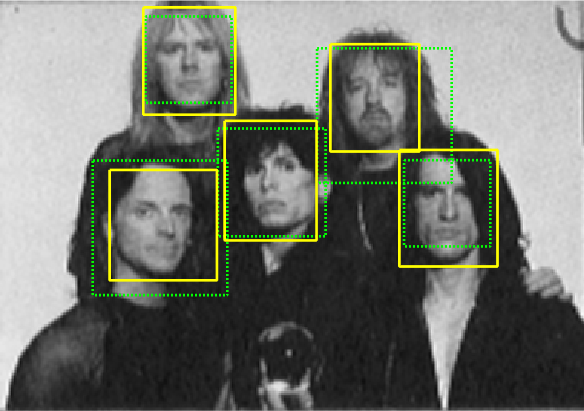
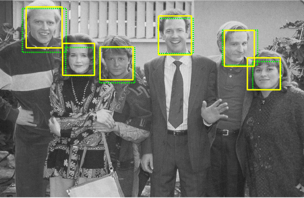
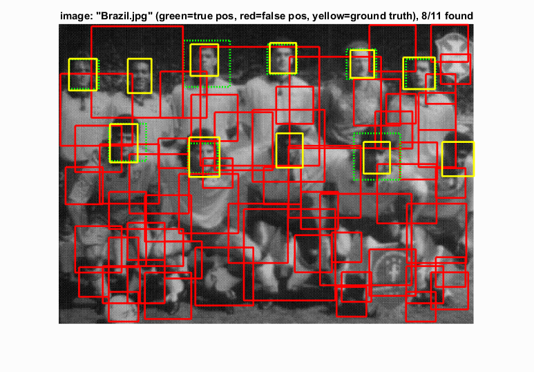
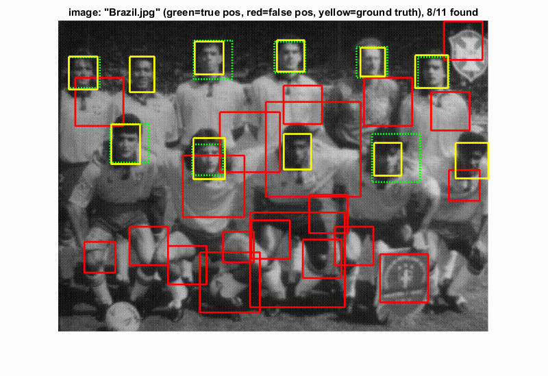
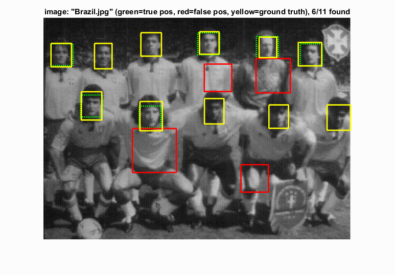
Example face detection
This project focused on the implementation of a sliding window face detector. The implementation utilizes HoG features in order to generate both positive and negative training examples. Once a classifier is trained with these examples, a sliding window detector along with HoG features can be used to detect faces within an image.
Algorithm Explanation
Positive Features
To detect a face within an image, we first need to figure out what a face looks like. To do this, we can take a training set of images that we know are faces, and compute HoG features for all of these faces. What this allows us to do is create a template for a "face" in HoG feature space. In this case, input images are grayscale 36x36 images of front facing faces. The algorithm for this is quite simple. We only have to compute the HoG features for the image using a cell size of 6 in this case, and then store these features in a single matrix of positive features.
% We do this for all input images
hog = vl_hog(image, cellsize);
features_pos(i,:) = hog(:);
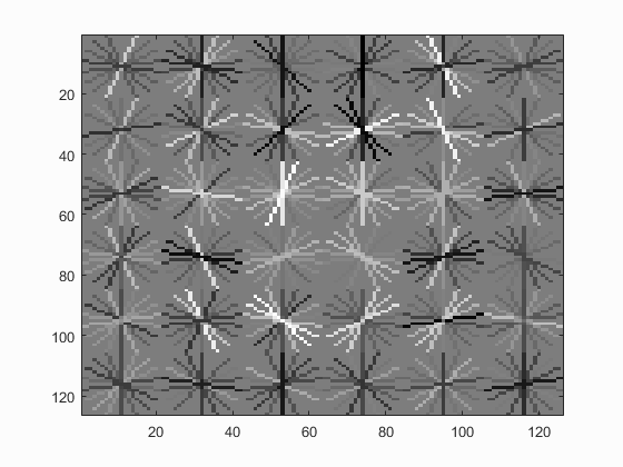
There weren't really many parameters to play with in this part of the pipeline, so the results and alogorithm were pretty straightforward. What this resulted in was the creation of a HoG "face" template which can be seen below
Negative Features
Next, in order to correctly classify objects as faces, we have to know not only what a face looks like, but also what a face doesn't look like. The algorithm for this was very similar to finding positive features, however, we needed to take multiple features from larger images, as our input images are not all perfect 36x36 images. In order to do this, I randomly sample a top left corner from a point within the image. I make sure that when extracting this random feature, the bounding box does not extend past the edge of the image.
Next, I compute the HoG feature for 36x36 pixel patch (based on the given template size.) The method takes in a parameter for how many negative features we want so the amount we should take for each image is simply our desired number divided by the size of the image set. Therefore, I take this number of random features from the image using the described algorithm and store them all in a single matrix of negative features.
% In this case, bbox_size is the width of our feature template (36x36)
r = randi([1, size(image,1)-bbox_size],1,1);
c = randi([1, size(image,2)-bbox_size],1,1);
hog = vl_hog(image(r:r+bbox_size-1, c:c+bbox_size-1), cellsize);
features_neg((i-1)*samp_each_image+j,:) = hog(:);
When calculating how many samples to take from each image, I opted to take the floor of the value in th case that it did not divide evenly. This results in the final feature matrix having slightly less than the desired amount. I decided this on the idea that we should preserve memory and compute the result slightly faster, as the number provided to the function can always be increased.
SVM Classifier
The next step in the pipeline is to actually create a learned classified based on these newfound positive and negative features. Since we have two matrices that have the same column dimension, we can simply append the two together in order to create our X for the svmtrain() function.
Next, we simply need to label them as positive or negative, which is quite simple. We know all the positive features are first, and all of the negative features follow. Therefore, I simply create a vector of all ones that is the same length as the total appended matrix. Then, I take the index following the last positive feature and set all values from that index to the end to -1, since that is where the negative features are located. This creates the needed Y vector for the svmtrain() function. Finally, we can utilize vl_svmtrain() with a best lambda of .0001 to calculate the w and b parameters of our classifier.
The only real free parameter that needed tuning in this section was the lambda parameter for the svmtrain() function. After some trial and error, I found that the consistenly best lambda value was around .0001. However, the lambda value didn't always seem to have a large effect as long as it was relatively small. More variation in the results seems to have been a result of the random negative feature generation rather than the lambda values. A table of results below shows some different Average Precisions based on different lambda values.
| Detector Precision (Threshold = 0) | |
|---|---|
| Lambda | Average Precision |
| .001 | 84.3% |
| .0005 | 85.1% |
| .0001 | 87.9% |
| .00005 | 86.0% |
Sliding Window Face Detector
The final piece of the face detection pipeline was the actual detector. Simply put, this detector is a sliding window detector that takes an image, calculates the HoG feature, then looks at patches of HoG cells to classify them as a face or not a face.
I first started with a detector that operates at a single scale. First, I calculate the HoG feature for the entire image. Next, now that I have a number of HoG feature cells, I "slide" a window over these cells and extract a range of them. In this case, we want the extracted features to match the size of the template from the original classifier. In this case, we utilized 36x36 pixel blocks that generated 6x6 cells of HoG features. For this reason, we utilize a window size of 6x6 HoG cells in the sliding detector.
The next step is to utilize the W and B from the classifier in order to classify the HoG feature for the given patch. If the classifier result is greater than a specific threshold, the location of the feature can be appened to the list of bounding boxes. This is done by using the coordinate as the top left corner of a bounding box. Since we have to convert HoG feature space back to image coordinates, some calculations are required to extract the actual pixel position. Since the cell size for our HoG feature is known, we can simply multiply the current cell number minus one, by the given cell size. Then, the width and height of the bounding box is simply the template size that was provided by the feature parameters.
The final step in the process is to perform non-maximum suppression. This is done simply to remove potential duplicate matches. Since a sliding window is being used, a small window slide may detect the same face many times. By performing non-maximum suppresion, we can ensure that bounding boxes overlap as little as possible, and the fewest number of confident detections are returned.
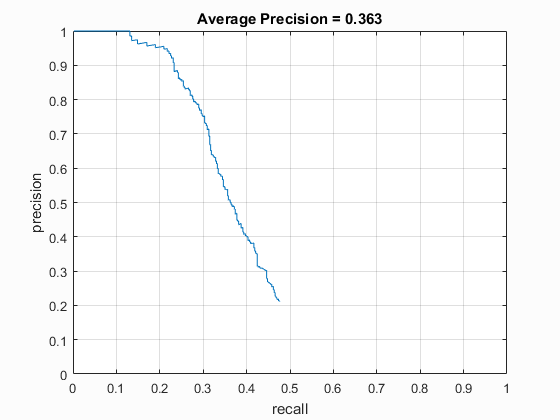
Without utilizing multiple scale detection, the Average Precision reported by the face detector was only about 36.3%. The poor results are attributed to the fact that faces were only being detected at a single scale. Larger or smaller faces would go unnoticed by the detector, therefore multiple scales are required to improve precision.
Multiple Scale Detection
To greatly improve the results of the sliding window detector, multiple scales for the sliding window are utilized. This only involves some minor changes to the code. Firstly, for every image, rather than calculating the HoG feature once, we must calculate the HoG feature once for each provided scale. This involves simply resizing the image to be a factor smaller than the original image before calculating the HoG feature. This is done so that very large images or faces are more easily detected. The size of the sliding window may remain constant, but by shrinking the image down, the sliding window can cover a larger area of the image, and thus detect larger faces. In this case, larger just means more pixel area.
The other necessary change for the code to operate at multiple scales is after a face has been confidently detected. In this case, it is necessary to convert from our HoG feature coordinate back to our actual image coordinate. In the single window, size our scale was 1, it had no effect on the image coordinate. However, when the image is scaled, it is necessary to retain the correct dimensions of the bounding box based on the scale of the image. This is easily done by taking our template width and dividing it by the current scale when calculating the width and height of the bounding box, as well as the top left corner. This ensures that pixel coordinates are mapped correctly, and bounding boxes are correctly placed and sized.
%This is done for each window of HoG cells
%c_size is the HoG cell size (6)
%t_size if the HoG template size (36)

hog_cell = hog(j:j+c_size-1,k:k+c_size-1,:);
% Flatten the hog cell
hog_cell = reshape(hog_cell, [1, c_size*c_size*31]);
conf = hog_cell*w + b;
% Save features that are confidentaly classified as faces
if conf > threshold
    cur_confidences = [cur_confidences; conf];
    cur_x_min = ((k-1)*c_size+1)/scales(s);
    cur_y_min = ((j-1)*c_size+1)/scales(s);
    bbox = [cur_x_min, cur_y_min, cur_x_min+t_size/scales(s), cur_y_min+t_size/scales(s)];
    cur_bboxes = [cur_bboxes; bbox];
end
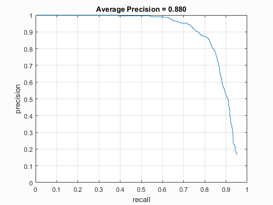
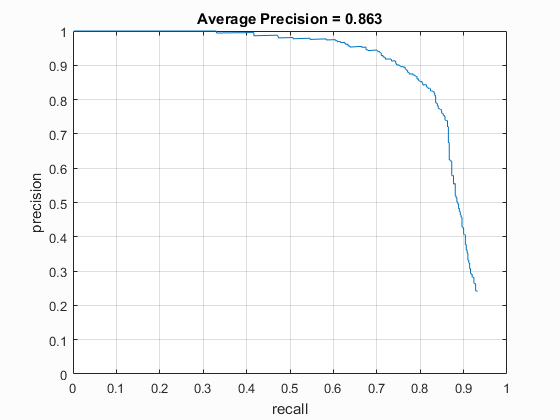
The threshold used above was a very important parameter for the Average Precision of the detector. It was very clear that using too high of a threshold resulted in lower precision, because some faces did not produce quite a confident enough result. This made many faces be passed over and not classified correctly. On the other hand, utilizing too low of a threshold resulted in far too many false positives. Therefore, a proper threshold was somewhere in the middle. I found that the best average precision was around 87%, and the best threshold for this precision was somewhere around 0. The fluctuations due to the negative feature generation made it difficult to pinpoint a hard value. However, I preferred in general the higher threshold. This was due to the fact of the precision being relatively similar, within 2% or so, while having many less false positives. In this case, I would prefer less false positives over a 1-2% gain in precision.
| Detector Precision (Viola-Jones Scales) | |
|---|---|
| Threshold | Average Precision |
| -1 | ~85.5% |
| 0 | ~87% |
| 1 | ~84.9% |
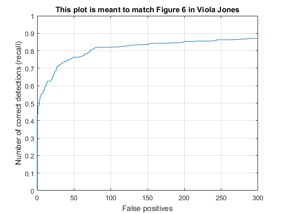
Another important element in this detector was the image scaling. I experimented a fair amount with the different scales that can be applied to the image. I first decided to simply try scales from 1 down to .1 in increments of .1 for a total of 10 scales. The accuracy fluctuated a fair amount with these scales and a threshold of zero, ranging anywhere from 84.6% to 87.9%. I then decided to utilize the scales suggested in the Viola-Jones paper, which started at 1, with each subsequent scale being 1.25 times smaller than the last. This resulted in a range of precisions from 85% to 88%. The two scales were not extremely different, so this wasn't very suprising that they produced similar results.
Results
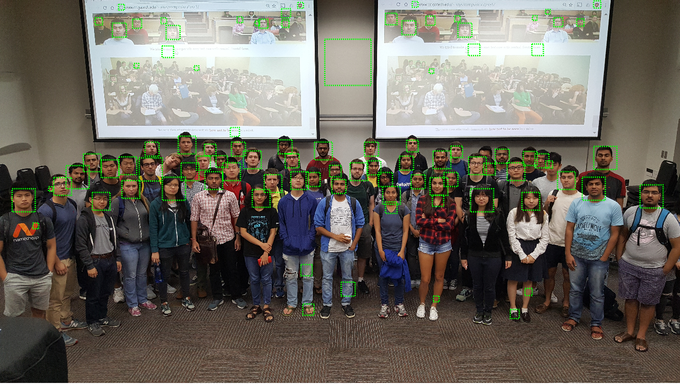
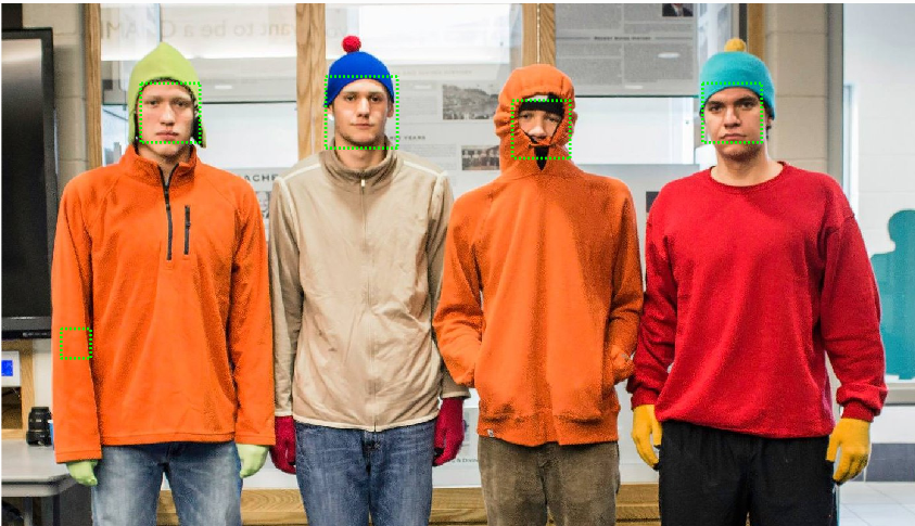
In the end, I was able to achieve accuracy within the range of 84-88% consistently without any of the extra credit. I found that the best threshold for the test set was generally around 0, though it produced too many false positives for my liking as far as the visualization images go. In the generation of some of the results below, I decided to use a slightly higher threshold to eliminate some of these false positives. However, I have also included the precision-recall and false positives graphs for my best performing pipeline.