Raj Prateek Kosaraju

Get Positive Features

Extracting the positive features was fairly simple. Just iterate through all the positive examples(of faces) and use vl_hog to extract features. We then simply save these features in our features_pos array to train our classifier later.

The matlab code to do the same is provided below:

for imageNum = 1:num_images
    cur_image = im2single(imread(fullfile( train_path_pos, image_files(imageNum).name)));
    vl_hog_feats = vl_hog(cur_image, feature_params.hog_cell_size);
    features_pos(imageNum,:) = reshape(vl_hog_feats,[],1,1);
end

Get Negative Features

For negative features, we take images which we know have no faces and randomly select patches from the images to extract features from. We keep extracting features from random patches for every image until we have enough negative features.

for sample = 0:num_samples-1
    imageNum = mod(sample,num_images)+1;
    cur_image = im2single(rgb2gray(imread(fullfile( non_face_scn_path, image_files(imageNum).name))));
    L = feature_params.template_size;
    [n m]= size(cur_image);
    crop = cur_image(randi(n-L+1)+(0:L-1),randi(m-L+1)+(0:L-1));
    vl_hog_feats = vl_hog(crop, feature_params.hog_cell_size);
    features_neg(sample+1,:) = reshape(vl_hog_feats,[],1,1);
end

Training the classifier

I used the vl_feat's svm method to train a linear SVM on the positive and negative features. This would return w and b, which we can later use to classify features as faces or non-faces with some confidence. Used a LAMBDA of 0.0001 as this gave the best results.

X = (cat(1,features_pos, features_neg))';
Y1 = ones(1, size(features_pos,1)) ;
Y2 = zeros(1, size(features_neg,1)) -1;
Y = cat(2,Y1,Y2);
[w b] = vl_svmtrain(X, Y, 0.0001) ;

Run Classifier on test images

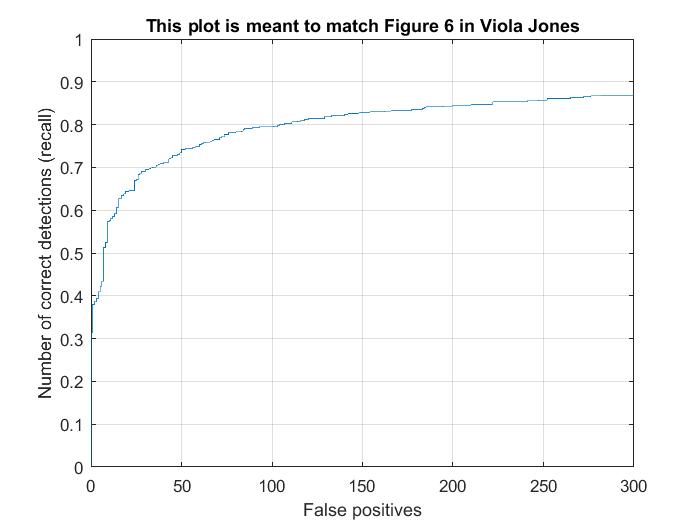
To run the classifier on the test images, we use a sliding window approach with a particular step size. We check if each of these steps is a face or not, using our trained SVM. I used a threshold of 0.65 - so all steps which had a confidence more than 0.65 using the trained SVM were classified as a face. Non-maximum suppression is used to remove repeitions in boxes of detected faces. I also performed this at multiple scales - begining at the full image and resizing by a factor of 75% each time. The results obtained are detailed in the next section.

Results

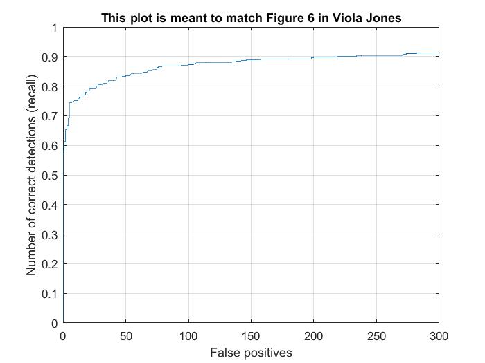
I ran the pipeline multiple times with various step sizes. I fixed LAMBDA at 0.0001 as this seemed the most effective. All of the following results were run with multiscale algorithm. The confidence threshold was set to 0.65 to achieve the best results.

Step Size = 6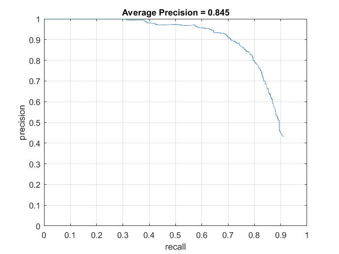
Step Size = 4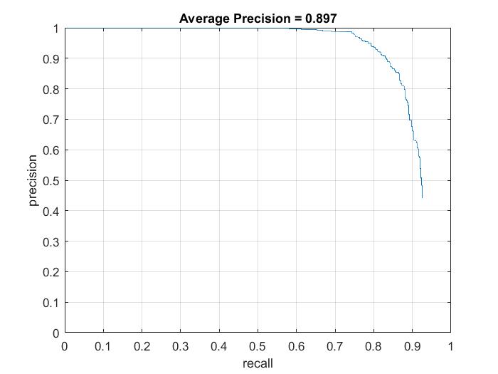
Step Size = 3

The max precision I've achieved using the various step sizes is 89.7% (from step size of 4). It's easy to see that as the step size decreases, the results seem to get better in general. However, they seem to plateau at around 90% and very fine tuning of hyper parameters may be needed to get better past this range.

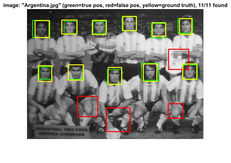
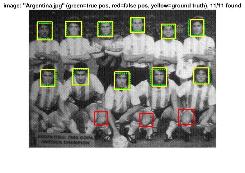
An analysis into the false positives showed that most false positives seem to have arised because of some bright, seemingly oval shaped figure in the image - causing the classifier to think it could be an image. I suspect that if we could somehow process color features more accurately, this could be avoided. The below picture illustrates this.

Above & Beyond

I tried to improve upon my best results above by trying these following approaches.

Mined more negatives

I modified my code so that it considers the false positives more from the training set. I first trained the classifier and then retrained it by adding the false positives to the negative features list again - essentially giving them more weight. This was also suggested by Prof. Hays on Piazza. The code to do this is as follows:

new_features_neg = features_neg;
for featureNum = size(features_pos,1) :  size(features_pos,1)+ size(features_neg,1)
    if confidences(featureNum)>0
        cur_feat =  features_neg(featureNum-size(features_pos,1),:);
        new_features_neg = [features_neg;cur_feat];
    end
end
features_neg = new_features_neg;

%retrain
X = (cat(1,features_pos, features_neg))';
Y1 = ones(1, size(features_pos,1)) ;
Y2 = zeros(1, size(features_neg,1)) -1;
Y = cat(2,Y1,Y2);
[w b] = vl_svmtrain(X, Y, 0.0001) ;
 

This improved prevision by approximately 2% to 87% while using step size of 6 and LAMBDA = 0.0001. This is particularly useful in scenarios where we have only a limited number of negative exmaples - we can utilize the false positives to give them more weight in the negative examples fed to the classifier.

Find and utilize alternative positive training data.

I added the code required to consider the mirror reflection of positive examples as well, thereby resulting in twice the number of positive features. This also resulted in an increase in precision by approximately ~1.5% (there is also some randomness involved) and gave results in the range of 86%. The code to do this is as follows:

    flipped  = flip(cur_image,2);
    vl_hog_feats_flip = vl_hog(flipped, feature_params.hog_cell_size);
    features_pos(imageNum*2,:) = reshape(vl_hog_feats_flip,[],1,1);