Si Chen

Example of a right floating element.

Positive & Negative Training Examples

To get positive training examples, I simply ran vl_hog on the provided images of faces and used the resulting HoG templates as my positive features To get negative examples, I sampled 10,000 crops of non-face images at random, used vl_hog to produce a HoG template, and used those as my negative features.

Training the Classifier

To train the classifier, I concatenated my positive and negative features and created labels for them accordingly, using +1 to represent positive and -1 to represent negative. Then, using vl_svmtrain, I trained an SVM which output the weight and bias terms.

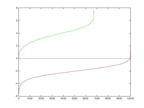
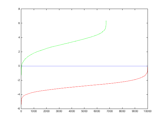
Here are the results of this classifier on the training data:

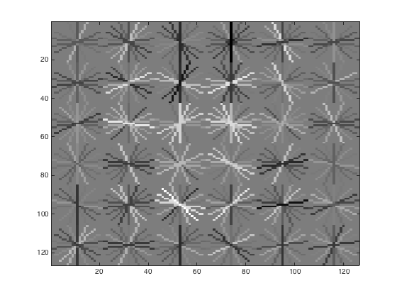
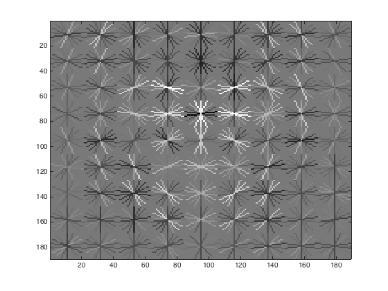
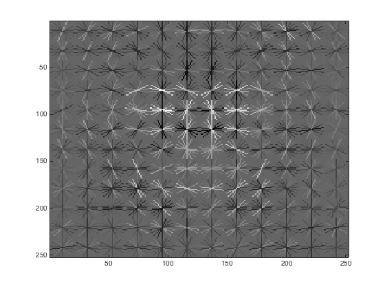
This is what the visualization for the HoG face template looks like:

With a HoG cell size of 6, the initial classifier performance on train data:

accuracy: 0.999

true positive rate: 0.401

false positive rate: 0.000

true negative rate: 0.598

false negative rate: 0.001

With a HoG cell size of 4, the initial classifier performance on train data:

accuracy: 0.999

true positive rate: 0.400

false positive rate: 0.000

true negative rate: 0.598

false negative rate: 0.001

With a HoG cell size of 3, the initial classifier performance on train data:

accuracy: 0.999

true positive rate: 0.401

false positive rate: 0.000

true negative rate: 0.598

false negative rate: 0.001

Testing the Classifier

To test the classifier, I had to use a sliding window approach to get the small patches across an image's HoG template. I then used the weight and bias terms to create a confidence value with the patch. For each image, the classifier was run at multiple scales to output bounding boxes for the faces at different scales. I did this at 6 scales, with each scale .8 the size of the previous image size. Non_max_supr_bbox removed duplicate detections of the same face at slightly different scales and locations.

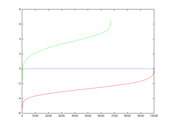
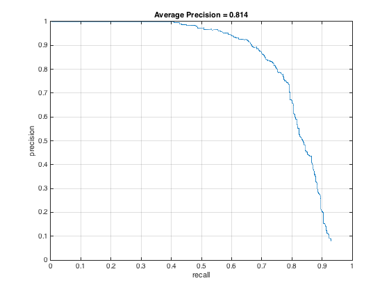
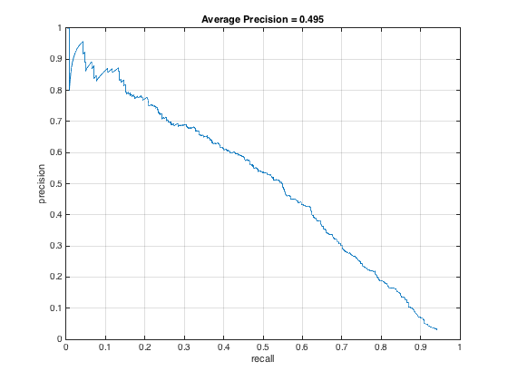
Trying different threshold values was quite important as well. Here is the precision recall curve for the threshold = .5, which yielded no more than 20 final bounding boxes:

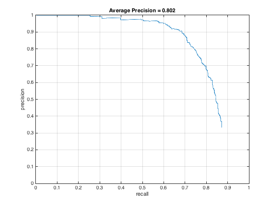
Alternatively, here it is for threshold = .2, which yielded 20 boxes on average:

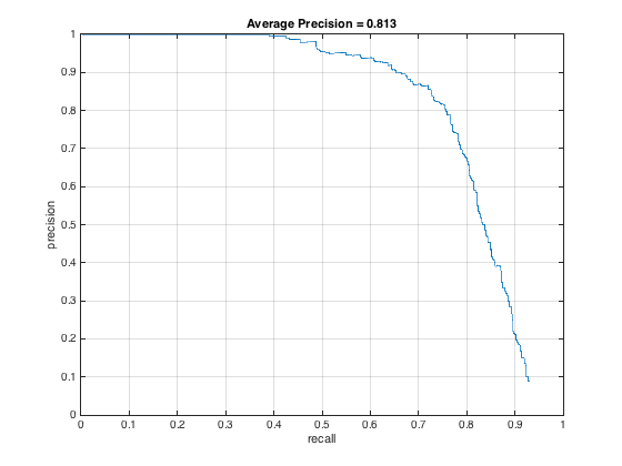
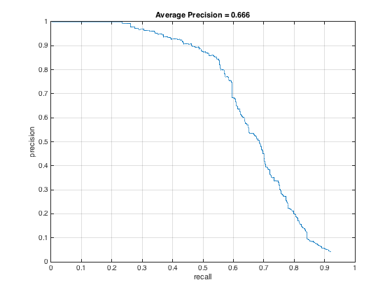
And, here it is for threshold = 0, produced the best PR curve:

Of course, the lower the threshold, the more bounding boxes produced. Setting the threshold too high actually hurt precision and recall. And finally, here it is for threshold = -.2 and -.5 respectively

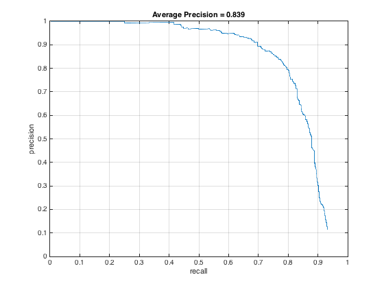
I originally had my downsampling rate at .8 and only downsampled 6 times, but after switching to .9 and downsampling 12 times, my PR curve changed to this, an incremental improvement:

Example of detection on the test set:

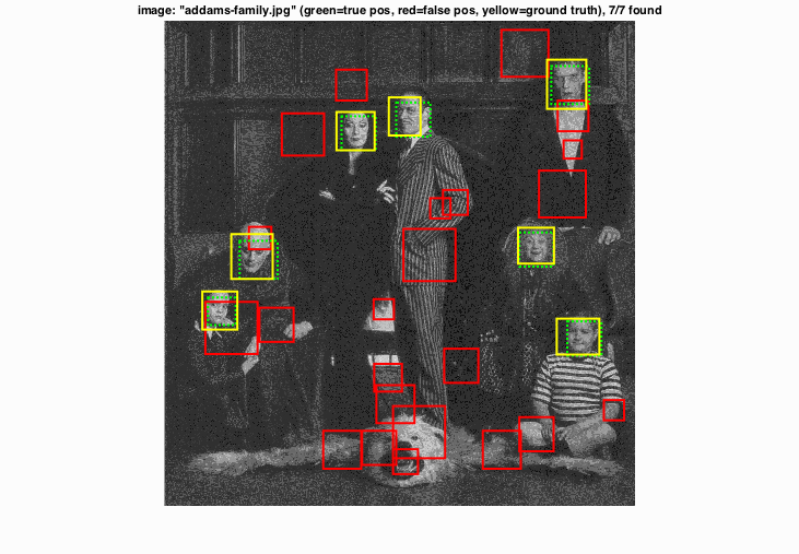
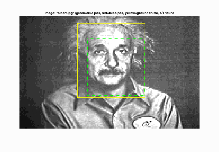
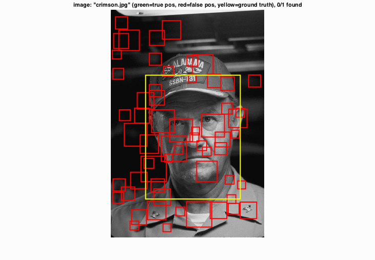
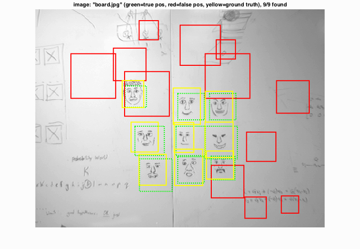
To explain my results, I've shown a few different success and failure cases above. On the top left, while I find all the appropriate faces, I also find quite a few non-faces that are clearly just image patches that are slightly noisy. On the top right, it's a complete success case with no extraneous red boxes. On the bottom left, after looking at the resolution of the image (I had naively assumed all my testing data would be about the same size) that my downsampling method was not enough of a scale change on particularly large images. Had I realized this earlier, I might've changed my code so downsampling progressed even more on larger photos while it remained smaller on smaller photos. On the bottom right, again, all the faces are found, but patches of whiteboard are also labeled as faces too which baffles me.

Extra Credit

Find and utilize alternative positive training data. You can either augment or replace the provided training data.

In this portion, I augmented the number of positive training examples through the following methods:

1. Mirroring the image along the the x-axis.
2. Rotating the image at 3 different degrees: 90, 180, 270.
3. Image jitter: where noise is randomly added to the image.

For image jittering in particularly, playing around with the parameters of the noise functions to ensure that the images weren't rendered completely noisy was important due to the small size of the images. Below are examples of what each image augmentation method produced, given this original image:

These images show on the first row the effect of mirroring and rotating at 90, 180, and 270 degrees. The second row shows the effect of adding different types noise to the images: poisson, gaussian, salt and pepper, and speckle.

Doing this affects the training accuracy:

Initial classifier performance on train data:

accuracy: 0.987

true positive rate: 0.852

false positive rate: 0.007

true negative rate: 0.135

false negative rate: 0.006

The result of adding additional positive training data is shown in the below PR curve. After looking through the test dataset, I realized that not many faces were rotated, so I took that section out of the augmentation. That led to the PR curve on the middle, which is better, but still not as good as I had hoped. Then, I tried to remove the jittering with noise, which is what's shown in the PR curve on the right. That gets us back to pretty much our starting point. It's interesting that in this case, the addition of positive training examples didn't improve PR.

Along this line of thinking, I wondered if the issue was an imbalance in the proportion of positive-negative training examples, especially since even just mirroring increases the number of positive examples by a factor of 2. To see if maintaining the ratio would help, I increased the number of negative training examples from 10,000 to 20,000 and only had mirroring as the data augmentation. As shown below, the average precision doesn't change as a result from this, though the precision at lower recall rates increases.

HoG

In this portion, I expanded upon my SIFT code from project 2 to create the HoG features. I had some weird behaviors in creating this feature though--I got an accuracy of 100% on my training data, but a false positive & negative and true positive & negative rates of all 0. So, clearly there were issues with this. Looking deeper, I found that I would get NaNs in my features (which means at some point I was dividing by 0), but I never got to the root of the problem. You can still see all my code in the section I've specifically commented that contains the HoG code.