Shing Shin Cheng

Sampling HoG features from cropped positive face images

The step is straightforward since the images are readily cropped to the template size (36 pixels by 36 pixels). Each of these cropped face images is converted into a hog feature, which is a 3-D matrix. The third dimension has 31 feature components. The number of column and number of row of each of the 31 feature component is equivalent to the quotient when the template size is divided by the Hog cell size. In other words, each entry in each of the 31 2D matrices of the HoG feature represents number of actual image pixels that is equivalent to the user-specified cell size. vl_hog function is used to obtain the HoG feature which is then reshaped into a row vector for each image.

get_positive_features.m

templatesize = feature_params.template_size;
cellsize = feature_params.hog_cell_size;
hogfeature = templatesize/cellsize;
features_pos = [];  
imagelist = dir( fullfile(train_path_pos, '*.jpg'));
num_image = length(imagelist);
    for i=1:num_image
       pos_crop_image_paths{i} = fullfile(train_path_pos, imagelist(i).name);
       image = single(imread(cell2mat(pos_crop_image_paths(i))));
       hog = vl_hog(image,cellsize);
       features_pos(i,:)= reshape(hog,[1 hogfeature^2 * 31]);
    end

Sampling HoG features from random negative scene images without faces

The scene images without faces provided are of multiple random dimensions. The image is selected for further processing based on the outcome of a random organization. The image is divided into patches of the size of the templates (36 by 36 pixels). These patches are randomly selected to be converted into HoG features. A cap is set so that patches can only be selected from 50 distinct rows and columns from one image. The number of negative samples required is 10000. Throughout the different for loops in the code, the cumulative number of HoG features are checked to ensure the negative data sampling process stops once the required number of 10000 is achieved.

get_random_negative_features.m

image_files = dir( fullfile( non_face_scn_path, '*.jpg' ));
num_images = length(image_files);
t = randperm(num_images);
featuresperimage = 50;

templatesize = feature_params.template_size;
cellsize = feature_params.hog_cell_size;
hogfeature = templatesize/cellsize;

j = 1;
for i=1:num_images
     if j>num_samples
            continue;
     end
   
   neg_image_paths{i} = fullfile(non_face_scn_path, image_files(t(i)).name);
   image = single(rgb2gray(imread(cell2mat(neg_image_paths(i)))));
   
   if size(image,1)featuresperimage
       row = row(1:featuresperimage);
   end
   if length(col)>featuresperimage
       col = col(1:featuresperimage);
   end
   
   for m = 1:1:length(row)
       if j>num_samples
            continue;
        end
       for n = 1:1:length(col)
       if j>num_samples
            continue;
        end
   sample = image(row(indrow(m)):row(indrow(m))+templatesize-1,col(indcol(n)):col(indcol(n))+templatesize-1);
   hog = vl_hog(sample,cellsize);
   features_neg(j,:)= reshape(hog,[1 hogfeature^2 * 31]);
   j = j+1;
       end
   end
end

Training classifier

This is the most straight forward step in the project. The linear SVM classifier written for the previous project was implemented. There is no complications involved. The positive features and negative features are combined into one huge matrix and each row vector representing one HoG feature or one trained image is assigned a positive 1 or negative 1 value. Then vl_svmtrain is called to generate the w and b parameters based on the user-specified lambda, which is set to 0.0001 in the beginning.

step 3 in proj5.m

LAMBDA = 0.0001; 
X = [features_pos; features_neg];
Y = [double(ones(1,size(features_pos,1))) double(ones(1,size(features_neg,1)))*-1];
[w b] = vl_svmtrain(X', Y, LAMBDA);

Running the detector through the test images using the classifier

in this section, images are resized to many different scales (such as 1.3, 1.15, 1, 0.9, 0.8, 0.7, 0.6, 0.5) and at each scale, the images larger than the template size of 36 by 36 pixels are converted into HoG features. A patch, consisting of HoG cells that are of the size "template size/cell size", that represents a 36 pixel by 36 pixel image template is checked using the classifier for a score. A threshold is also set such that only the patches that have scores beyond the threshold will be remembered as detected faces. The threshold is set as 0.6 in the beginning. The step size in unit of pixels is limited by the cell size. The step size can be made larger for faster computation time. For most of the tests that I perform, my cell size is set to 3 pixels. The step size, which is equivalent to the cell size, is also 3 pixels. With an average computation time of 9.5 minutes for run_detector.m based on all the tests I performed, this step size is optimal enough to lead to high enough precision and satisfactorily small computation time. The pixel locations of the detected "faces" are remembered. After one test image (of all the different scales) is processed, all the detected faces are filtered to remove duplications.

run_detector.m

for i = 1:length(test_scenes)
      
    fprintf('Detecting faces in %s\n', test_scenes(i).name)
    img = imread( fullfile( test_scn_path, test_scenes(i).name ));
    img = single(img)/255;
    if(size(img,3) > 1)
        img = rgb2gray(img);
    end
    
    scale  = [1.3 1.15 1 0.9 0.8 0.7 0.6 0.5];
    
    cur_bboxes = zeros(0, 4);
    cur_confidences = zeros(0,1); 
    cur_image_ids = cell(0,1);
    for j = 1:length(scale)
    testimage = single(imresize( img, scale(j)));
        if size(testimage,1)< templatesize || size(testimage,2)< templatesize
            continue;
        end
    hog = vl_hog(testimage, cellsize);
    hogrow = size(hog,1);
    hogcol = size(hog,2);
        for RR = 1:hogrow-hogfeature+1
            for CC = 1:hogcol-hogfeature+1
            patch = hog(RR:RR+hogfeature-1,CC:CC+hogfeature-1,:); 
            patchvec = reshape(patch,[1 hogfeature^2 * 31]);
            score = w'*patchvec'+b;
                if score>thres
                point(1) = round((CC-1)*cellsize/scale(j)+1);
                point(2) = round((RR-1)*cellsize/scale(j)+1);
                point(3) = round(point(1)+templatesize/scale(j)-1); 
                point(4) = round(point(2)+templatesize/scale(j)-1); 
                cur_bboxes = vertcat(cur_bboxes, point);
                cur_confidences = vertcat(cur_confidences,score);
                cur_image_ids = [cur_image_ids;test_scenes(i).name];
                end
            end
        end
    end
    
    %non_max_supr_bbox can actually get somewhat slow with thousands of
    %initial detections. You could pre-filter the detections by confidence,
    %e.g. a detection with confidence -1.1 will probably never be
    %meaningful. You probably _don't_ want to threshold at 0.0, though. You
    %can get higher recall with a lower threshold. You don't need to modify
    %anything in non_max_supr_bbox, but you can.

    [is_maximum] = non_max_supr_bbox(cur_bboxes, cur_confidences, size(img));

    cur_confidences = cur_confidences(is_maximum,:);
    cur_bboxes      = cur_bboxes(     is_maximum,:);
    cur_image_ids   = cur_image_ids(  is_maximum,:);
 
    bboxes      = [bboxes;      cur_bboxes];
    confidences = [confidences; cur_confidences];
    image_ids   = [image_ids;   cur_image_ids];
end

Extra Credit

An additional dataset from LFW face database is downloaded and used to increase the number of positive trained faces that would be used to train the SVM classifier. The same get_positive_features function is called to process the images from this database. Additional few lines of codes are written to process these images which are organized in subfolders, different from how the caltech images are stored. The results from using this LFW database only and using both caltech and LFW images are stated in the results section.

Additional minor thing added

The HoG features from the positive and negative training sets are saved as features_pos.mat and features_neg.mat so that they do not need to be computed before every test. It should be noted that these mat files are specific for a particular HoG cell size and a particular number of negative samples. I also added tic and toc functions to calculate computation time for each step. When the code is run, the computation time for each step is displayed in the command window.

Results

1) Hog template size = 36 pixels; Hog cell size = 6 pixels; SVM classifier lambda = 0.0001; Scale = [1.3 1.15 1 0.9 0.8 0.7 0.6 0.5]; Confidence threshold = 0.6;

Number of negative samples	Precision
5000	0.767
10000	0.746
20000	0.759
50000	0.771

There is not any definitive conclusion on how varying the number of negative samples would affect the precision. Intuitively, it would be better to have more negative samples but it does not seem to help much or at all in some cases. It should be remembered that the more the samples, the longer the computation time.

2) Hog template size = 36 pixels; Hog cell size = 3 pixels; Number of negative samples = 10000; Scale = [1.3 1.15 1 0.9 0.8 0.7 0.6 0.5]; Confidence threshold = 0.6;

SVM classifier parameter, lambda	Precision
0.1	0.775
0.01	0.823
0.001	0.830
0.0001	0.832
0.00001	0.838

The decrease in SVM classifier parameter, lambda tends to increase the precision, albeit not by much beyond 0.01. There is however a significant improvement in precision from lambda=0.1 to lambda=0.01.

3) Hog template size = 36 pixels; Number of negative samples = 10000; SVM classifier lambda = 0.0001; Scale = [1.3 1.15 1 0.9 0.8 0.7 0.6 0.5]; Confidence threshold = 0.6;

HoG cell size	Precision
3	0.832
6	0.746
9	0.580

The HoG cell size affects many aspects of the code including the HoG feature size and the step size during detection process. As the HoG cell size decreases from 9 to 3, the precision increases by around 43%. If computation time is not a concern, a smaller HoG cell size would definitely be preferred.

4) Hog template size = 36 pixels; Hog cell size = 3 pixels; Number of negative samples = 10000; SVM classifier lambda = 0.0001; Confidence threshold = 0.6;

Scale	Precision
[1.3 1.15 1 0.9 0.8 0.7 0.6 0.5]	0.832
[1.3 1.15 1 0.9 0.8 0.7 0.6 0.5 0.4 0.3 0.2]	0.896
[1.3 1.15 1 0.9 0.8 0.7 0.6 0.5 0.4 0.3 0.2 0.1]	0.902

Each of the test images is resized into different scales to be processed for face detection. When the images are made very small, I actually get higher precision. In fact, I was able to achieve more than 90% precision in the third case.

5) Hog template size = 36 pixels; Hog cell size = 3 pixels; Number of negative samples = 10000; SVM classifier lambda = 0.0001; Scale = [1.3 1.15 1 0.9 0.8 0.7 0.6 0.5];

Confidence threshold	Precision
0.2	0.832
0.4	0.833
0.6	0.832
0.8	0.812
1	0.784

The confidence threshold is adjusted to vary the number of detected faces that would be remembered before the filtering step. The lower the confidence, the larger the number of image patches that are stored for filtering. Even though most of them are either duplicates or false positives, the precision would still increase, at least to a certain level, since the evaluation algorithm does not penalize false positives. In my case, any threshold lower than 0.6 does not help improve the precision.

6) Hog template size = 36 pixels; Hog cell size = 3 pixels; Number of negative samples = 10000; SVM classifier lambda = 0.0001; Scale = [1.3 1.15 1 0.9 0.8 0.7 0.6 0.5]; Confidence threshold = 0.6;

Data Sets	Precision
Caltech only	0.832
Caltech + LFW Face Training Data	0.818
LFW Face Training Data only	0.470

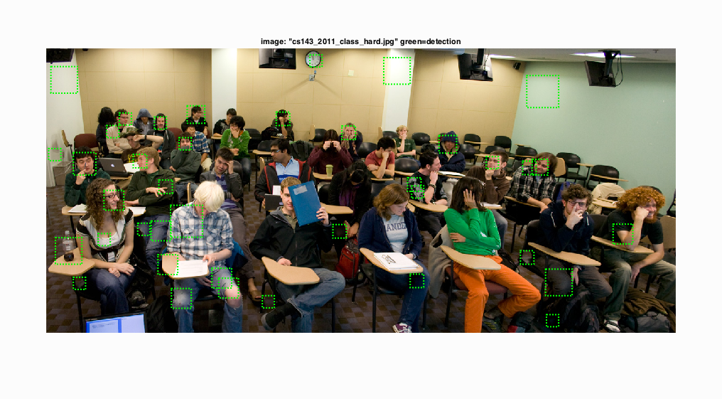
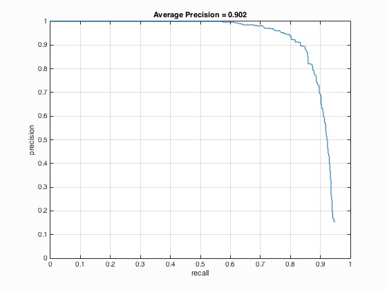
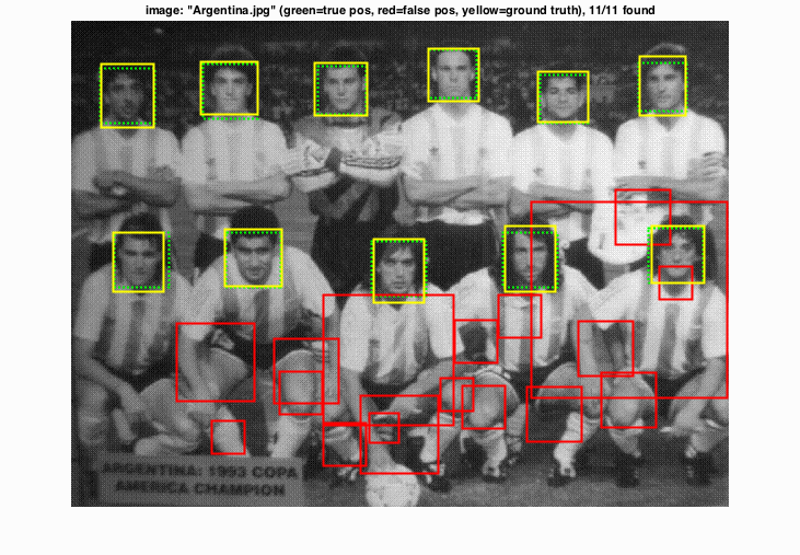
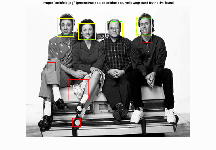
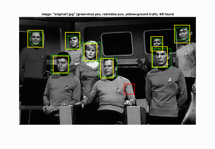
The test images below are achieved using the following parameters.

Hog template size = 36 pixels; Hog cell size = 3 pixels; Number of negative samples = 10000; SVM classifier lambda = 0.0001; Confidence threshold = 0.6; Scale = [1.3 1.15 1 0.9 0.8 0.7 0.6 0.5 0.4 0.3 0.2 0.1];

Precision Recall curve for the starter code.

Example of detection on the test set from the starter code.

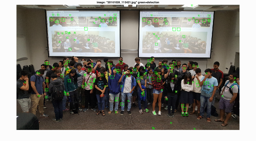
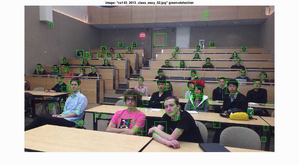
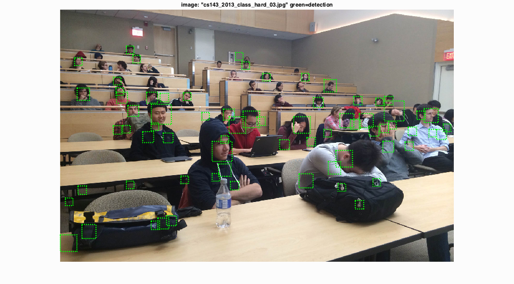
The class images below are achieved using the following parameters. There are a lot of false positives.

Hog template size = 36 pixels; Hog cell size = 6 pixels; Number of negative samples = 10000; SVM classifier lambda = 0.0001; Confidence threshold = 0.4; Scale = [1.3 1.15 1 0.9 0.8 0.7 0.6 0.5];

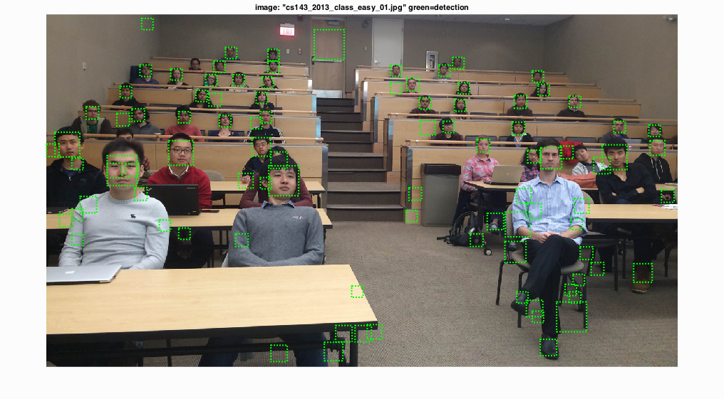
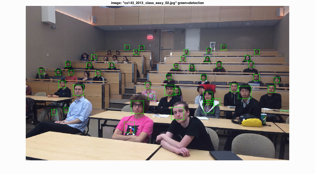
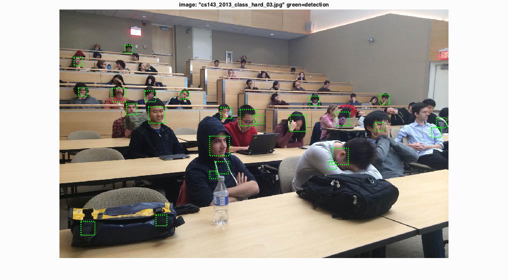
The confidence threshold was then set to 1.2 and the results are as follows with less false positives:

The following class images show how the students can avoid being detected by my algorithm.