CS 6476: Project 5 / Face Detection with a Sliding Window
Overview
In this project, we explore the Caltech Web Faces dataset of 6,713 cropped faces at a resolution of 36x36 pixels. The feature extraction process leverages the training dataset of positive face examples to compute HoG (histogram of oriented gradients) descriptors that, together with numerous negative examples partially taken from the SUN scene database, are used to train a linear SVM that classifies faces from non-faces. The final step of the detection pipeline moves a sliding window across the entire test image at multiple scales. HoG features are then collected and fed into the trained linear SVM that classifies each region inside the window as a face or a non-face.
Step 1: Positive and Negative Example Training
In the first step of the face detection pipeline, positive face examples with dimensions 36x36 were selected, and HoG features were computed from those images. Similarly, we extracted HoG features from the negative examples but performed random croppings across multiple scales to obtain a sizeable number of non-facial features. Most of the detection experiments for this project trained on a total of 20,139 positive HoG examples and 10,000 non-facial examples for a 2:1 ratio of positive to negative examples. Tuneable parameters in this stage were the HoG cell size, with smaller cell sizes resulting in increased detection accuracy, and the number of negative samples to include in the training set.

Fig. 1: Visualization of HoG features for a sample face image.
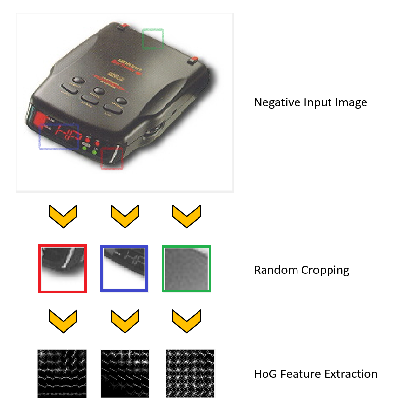
Fig. 2: Feature extraction of negative training examples.
Step 2: Training the Linear SVM Classifier
In this step, we train a linear SVM classifier with the labeled HoG features extracted from each training example. The parameter lambda, after some experimentation, was fixed to 1e-4 for all experiments. The output of the SVM training gives the weights w and bias term b. w is a column vector with dimension dx1, where d is a function of the HoG cell size c and template size t, computed as
Below are the HoG templates learned after training the linear SVM on cell sizes of 6, 4, and 3. From these images, we observe that smaller cell sizes are able to capture the finer details of the human face.
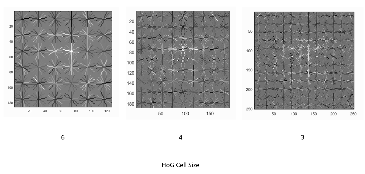
Fig. 3: Visualization of the learned HoG template.
Fixed training parameters used were lambda=.0001, number of negative samples = 10,000, template size = 36.
Step 3: Face Detection on the Test Set
The final step of the detection pipeline is straightforward. A HoG descriptor is computed for the the test image, and a multi-scale sliding window is passed through the entire image. Next, the trained linear SVM outputs a confidence value over the HoG features within each subwindow; values closer to +1 indicate a greater likelihood that a face is present, while values closer to -1 do not. By iteratively resizing the test image and passing a fixed-sized template across it, we obtain a sliding window detector that operates on multiple scales and outputs the bounding boxes corresponding to subregions with high confidence values. Finally, non-maximal suppression combines redundant, overlapping bounding boxes and, hence, contributes to a reduction in false positives.
Since the number of scales to resize the image on each pass of the detector influences the average precision achieved on the test set as well as the granularity of the bounding box dimensions, we measure this observation by comparing test-time performance to a single-scale detector across multiple HoG cell sizes of 3, 4, and 6. The results of the sliding face detector are displayed in the graph below (Fig. 4). For a HoG cell size of 3, note the drastic average precision increase when we use a 45-scale detector (89.3%) vs. a single-scale detector (33.5%).
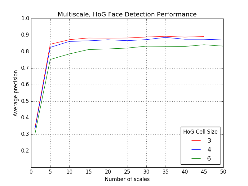
Fig. 4: Performance of the linear SVM-based sliding window detector on the CMU+MIT test set.
Fixed parameters: lambda=.0001, number of negative samples = 10,000, confidence threshold = 1.00, with data augmentation (random flips and blurs).
Results: Precision-Recall Curve and Sample Detections
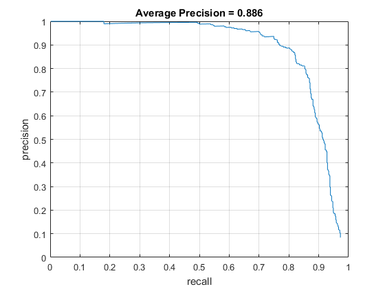
Fig. 5: Average Precision with HoG cell size of 4, data augmentation, confidence threshold of 0.90, number of scales = 45, and no hard negative mining.
The detector trained with this scheme makes many false positive guesses in order to increase its final average precision over all test images. This pattern is observed in the following sample detections (Fig. 6).
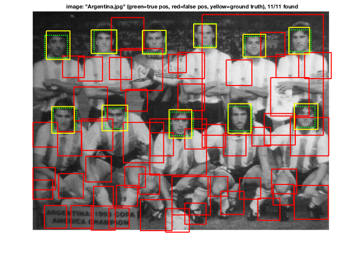
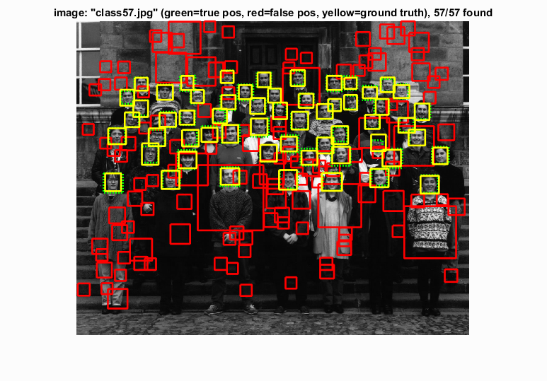
Fig. 6: While the ground truth faces are, in fact, being localized, many false-positive bounding boxes are also being generated from the HoG-based face detector.
However, we observe that in images with less "visual clutter" (large textureless regions, low scene complexity, etc.) and a small number of actual faces, bounding box localization performs well with few false positives.
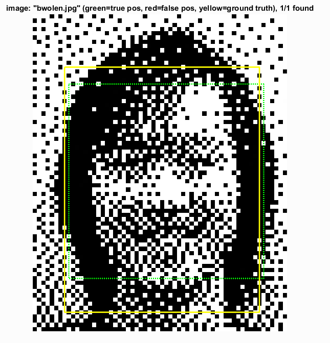
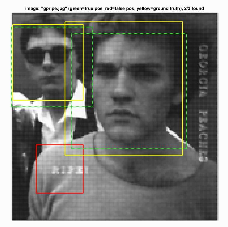
Fig. 7: Face detection in simple images.
Extra Credit #1: Positive Training Examples through Data Augmentation
Sometimes it's not enough to just normalize the images prior to training a classifier. We can benefit by applying some preprocessing operations like randomly flipping, rotating, and blurring images in an existing training set to produce more desirable positive examples with which to train the classifier. In this project, simply by extracting HoG features on top of randomly flipped and blurred training images (see Fig. 1) and using these as additional positive features to train the linear SVM, average precision saw a dramatic improvement of +10.3% on the 45-scale face detector in comparison to the one trained on the original 6,713 36x36 faces. The results are summarized in the graph below (Fig. 8):
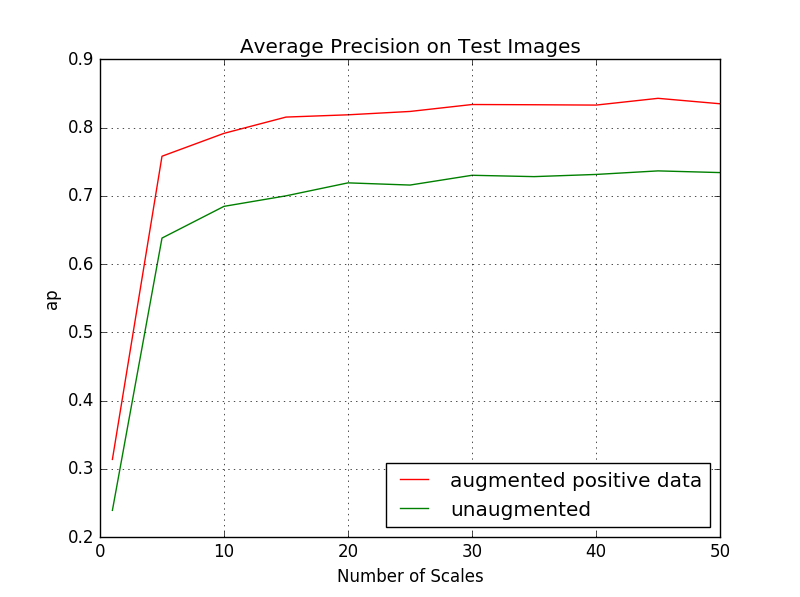
Fig. 8: Test-time performance of the object detector trained on augmented positive face examples from the Caltech dataset.
Parameters: HoG cell size = 6, template size = 36, SVM lambda=0.0001, total positive examples = 20139, number of negative samples = 10000, no hard negative mining, confidence = 0.8.
Extra Credit #2: Hard Negative Mining
As discussed in Dalal and Triggs 2005 (pg. 2), the process of hard negative mining trains an initial detector from existing positive and negative examples and runs this detector to identify false positive subwindows in negative training images known to be people-free. These false positives are then appended to the existing set of negative features, and we retrain the linear SVM in order to obtain refined weight and bias parameters.
I did not see as much an improvement in average precision using hard negative mining than with data augmentation discussed in the previous section. In fact, hard negative mining actually led to a 4.3% decrease in average precision (88.6% -> 84.3%), using the fixed parameters of the detection pipeline mentioned in Fig. 5. This observation can be explained with knowledge of the training dataset and the method of sampling negative HoG features. First, positive face examples retrieved from the Caltech dataset contained very little noise (Fig. 9), so we were confident that the HoG features fed into the SVM encoded actual human faces. Second, since negative features were already sampled randomly at multiple scales (see Fig. 2) from scenes known to be absent of human presence, mining legitimate "hard negatives" falsely classified to be faces would require meticulous adjusting of the confidence threshold parameter that, if not properly tuned, would more likely than not give noisy hard negatives which would decrease the final performance of the face detector. Third, as was discussed in class, hard negative mining is primarily beneficial if we lack enoughn negative training examples, which was not the case for this project. However, I observed that training on these hard negatives did reduce the number of spurious bounding boxes generated by the detector.
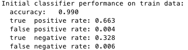

Fig. 9: Training statistics prior to hard negative mining with HoG cell size = 6, number of negative samples = 10000, total positive examples = 20139.
Extra Credit #3: Viola-Jones Face Detection
The baseline multiscale, HoG-based face detector has a tendency to propose many false positive bounding boxes (refer to Fig. 6). The Viola-Jones object detection framework implements a cascade architecture that chains a series of strong classifiers (created by boosting several weak learners into one) and is robust to false positives by rejecting regions of noninterest early in the cascade. The assumption behind this architecture is that the majority of sliding windows across an image do not contain a face, so only when every classifier in the cascade chain agrees the candidate might contain a face do we return a true positive. Hence, we may sometimes observe a reduction in run time since negative samples will fail fast in the cascade classifier. In fact, we observe a 10x speed-up during test time face detection with the Viola-Jones pipeline compared to the baseline HoG detector while still achieving similar values of average precision (Fig. 10).
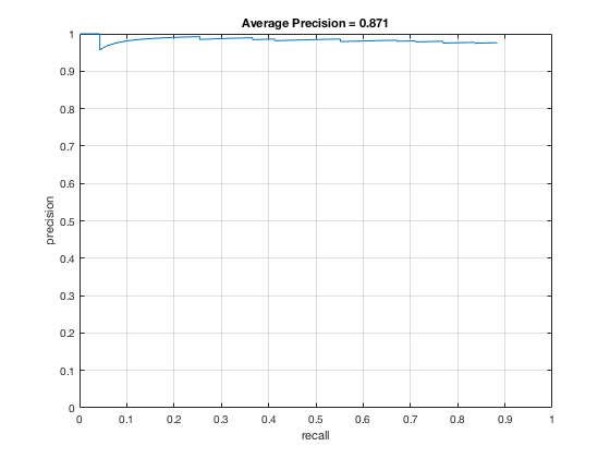
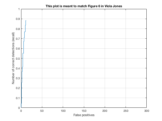
Fig. 10: Performance of the Viola-Jones detector on the MIT+CMU dataset. Precision-recall (left) and ROC curve (right).
A downside of the Viola-Jones detector is that as the number of classifiers in the cascade increases, in order to achieve high overall detection accuracy, each classifier in the chain must also have adequate detection ability. If a classifier incorrectly rejects a positive example early on, we cannot go back and correct the mistake, so it is important to have classifiers with low false negative rates. Despite high precision, the Viola-Jones detector, particularly the pretrained model I used, sometimes failed to localize bounding boxes around several obvious faces in the test set as a consequence of this conservative assumption with face detection.

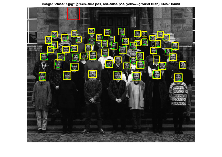
Fig. 11: Fewer false positives in comparison to HoG-based face detector.
Viola-Jones on Class Test Images
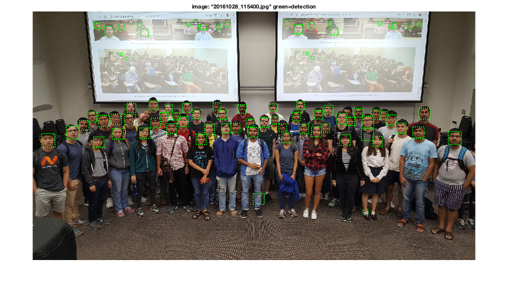
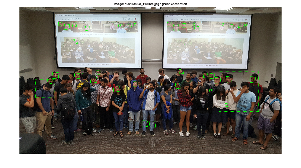
Fig. 12: Extra test images of students enrolled in CS 4496/6476.