Project 5 : Face Detection with a Sliding Window
Positive and Negative Features
In preparation for detecting actual faces, the SVM first need training to distinguish between correct and incorrect detections. So using the positive sample images of faces and negative images of non-faces, the HOG features for all training data were extracted. The positive samples were already 36x36, which required only setting the HOG cell size (initially set as 6). But for negative samples, random points were generated throughout the image, then used those random points as left-top-corner point for a 36x36 crop, which were again converted to HOG features of specified cell size.
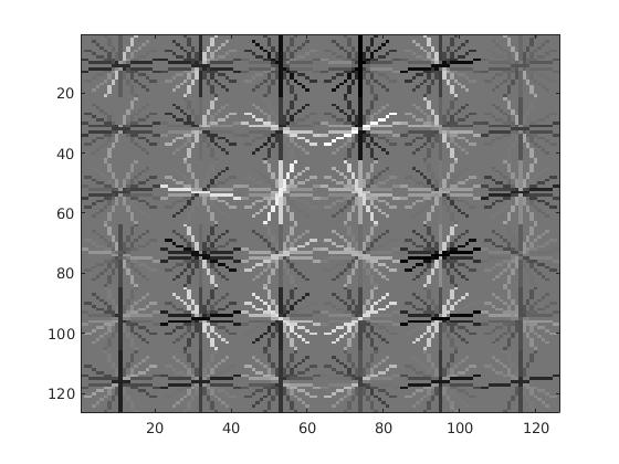
The image on the right is the visualization of the learned detector from the face images of size 36x36, with 6x6 HOG feature vectors. It's interesting to note the resemblance of a face contour shown through the image. Also, each cluster of vectors are symmetrical through the center vertical line (approximately 65 on the x-axis), much like a face. This indicates that the detector has successfully extracted significant structures of the faces given in the training example. However it's also worth noting that all the positive training images were centered and were front-facing faces, which might have facilitated the training process. Therefore, it is easily predictable that the detector will fail non-front-facing faces.
Sliding Window Face Detector
After training the SVM with positive and negative training samples, the test images were now ready to be detected for their faces. First the image is converted to HOG features using the same cell size used during training time. Then using the cell size as the size of the window, the HOG image features are converted to a single vector. This vector is then evaluated through the SVM trained beforehand. And if the score of the feature is greater than the threshold, the face is found! This process is repeated with varioius scales of windows because there are varied sizes of faces in the image. In order to vary the size of the bounding boxes, the size of the images are resized to various scales and the size of the window stays the same. This is inherently similar to varying the size of the actual bounding boxes, but easier to implement.
Parameter Tuning and Results
The implementation itself is not overly complicated, but the majority of the time were spent on parameter tuning. Some of the parameters I have toyed with include:
- SVM score threshold
- Number and size of scales
- Number of negative samples
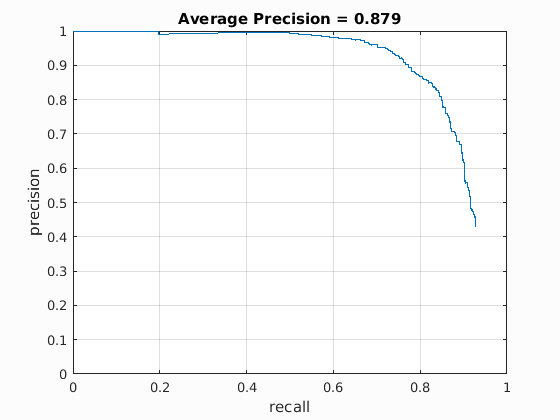
The average precision shown on the right is one of the best performances through parameter tuning. This is above the expected precision for a cell size of 6. The threshold were -0.25, image scales ranged from 0.05 to 1.05 with step size 0.05, and 670000 negative samples. In general, having more various scales improved precision, whereas the number of samples occasionlly improved precision, possibly due to the randomness of the negative feature extractor. So even with 10000 negative examples, an average precision of 86.6 were produced. The parameter I had most trouble were the SVM score threshold because intuitively having higher score values would be a stricter classifier which should eliminate false positives. However having lower threshold tend to produce higher precisions. I would suspect implementing hard mining the negatives would greatly improve this issue. Also, I have tried adjusting the lambda value for the SVM training, and the default value of 0.0001 produced the best average precision overall.
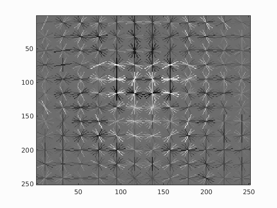
On top is an image similar to the first figure, but in more detail is the HOG descriptor using cell size of 3. Whereas the previous image with cell size of 6 was a rough contour of a face, this image shows more detail, including the contours of eyes, nose, and mouth. It's not suprising that the precision output 0.905 despite having less number of scales (scale step of 0.1, which is half of the original implementation above) to account for the slow computation time. This strongly suggests the importance of descriptive feature extraction, possibly more so than parameter tuning.
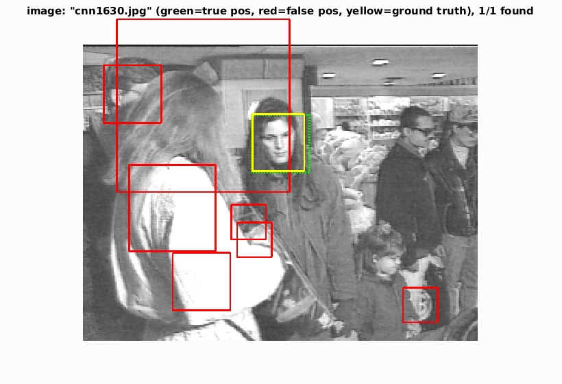
Interesting Example
As a last note, out of all the testing result images, I found the image above most interesting. There are 6 people in the image, but only one front facing person. All of the side view images were not detected, with an exception of the occluded side face on the left top corner. It's suprising how accurately the occluded face has been detected, which could be luck since all of the other side facing faces with no occlusions were not detected.