Project 5 / Face Detection with a Sliding Window
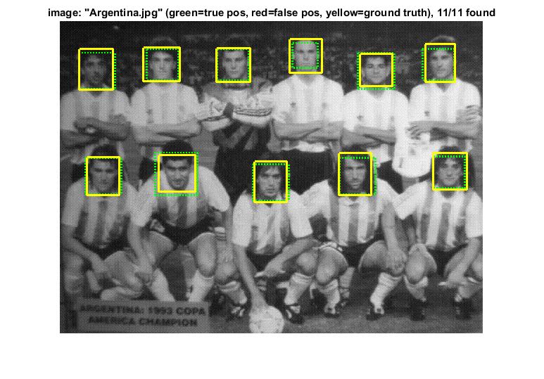
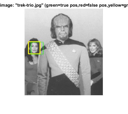
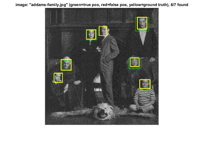
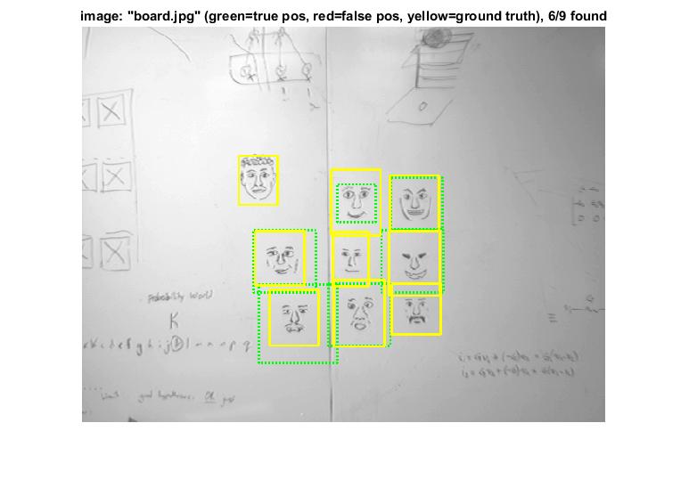
Example of a face detection.
The objective of this project is to detect faces in a image with SVM(Support Vector Machine) classifier trained on HOG(Histogram of Gradients) features. A sliding window is implemented to check for the faces. For better results, mirroring of positive features, different scaling for the sliding window and Hard Negative Mining is implemented. The major steps followed for face detection:
- Compute HOG features
- Train linear SVM classifier
- Retrain linear SVM using mined hard negatives
- Run the detector to find faces and non maximum suppression
Step 1: Compute HOG Features
The positive examples are presented and pre-cropped, whereas the negative examples need to be randomly obtained from images with no spaces. A random image is selected, then a constant number of random windows the same size as the postive features.
Here, the HOG features for the positive training images are mirrored to extend the trainign set. The number of negative features is set to 10000, to achieve fast implementation results, at the cost of a drop in accuracy.
Step 2: Train linear SVM classifier
All windows are converted to HoG space and are marked as either being face/non-face. The positive and negative features are labelled separately and are classified using a linear SVM. This is achieved using VL_Feat.
Step 3: Retrain linear SVM using mined hard negatives
To increase the accuracy, the negative features with the highest confidence are obtained. These are added to the negative set of images and the Linear SVM is retrained. Th confidence threshold is a free parameter here, to be tuned
Step 4: Run the detector to find faces and non maximum suppression
A sliding window is moved across the image to detect faces. The confidence of each window is calculated. Multi-scale sliding window is implemented, and non-maximal suppression is performed to find the most confident bounding box and to eliminate detection at multiple scales.
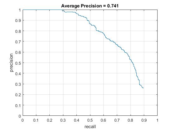
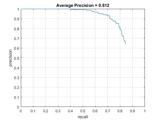
Without hard negative mining, the average precision was around 0.74. Only 10000 negative features were taken, to save on the computational time. The lambda for SVM training was set to 0.00005. With hard negative mining, the Average precision was approximately 0.812
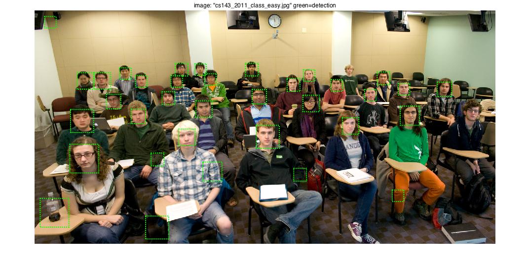
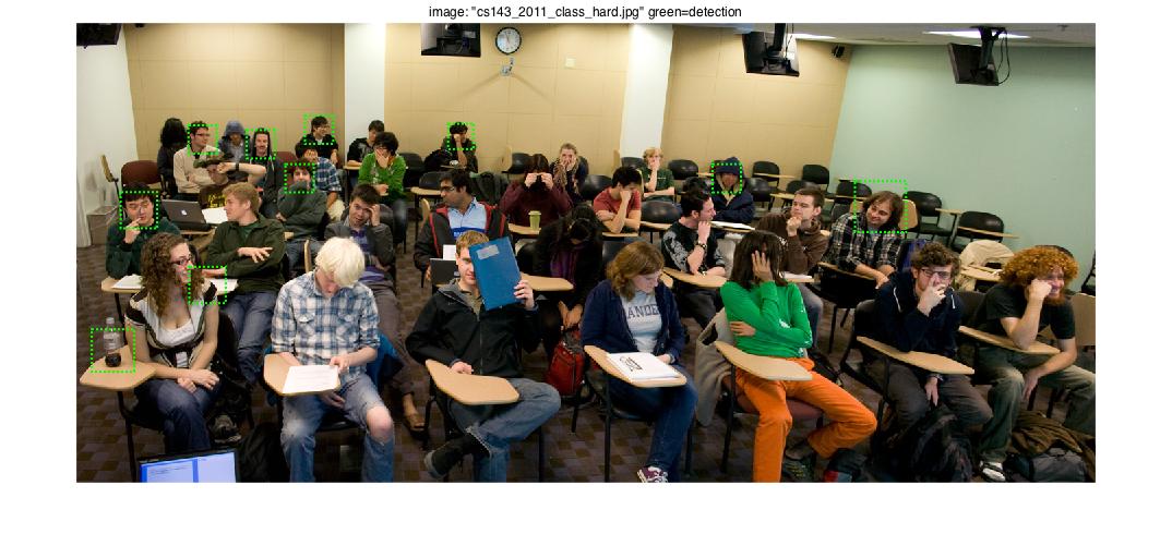
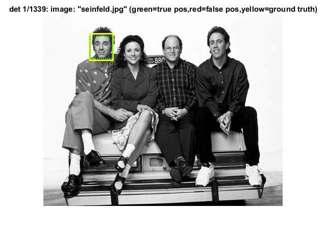
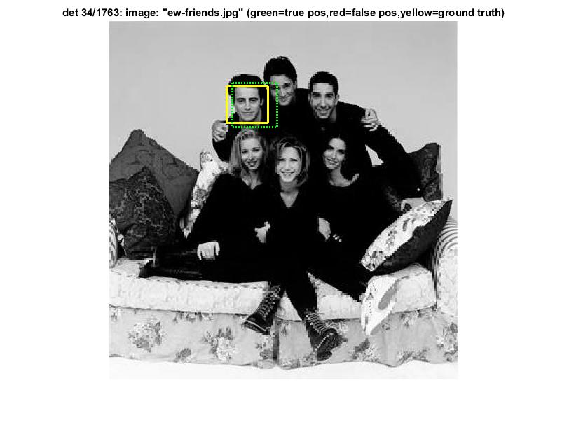
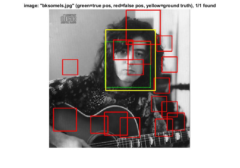
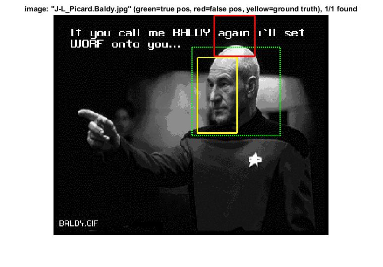
Sample Results
These results were obtained by using a cell size of 4 (as opposed to the default value of 6), and so the Average Precision was 0.86.
Face template HoG visualization for baseline implementation with varying cell size
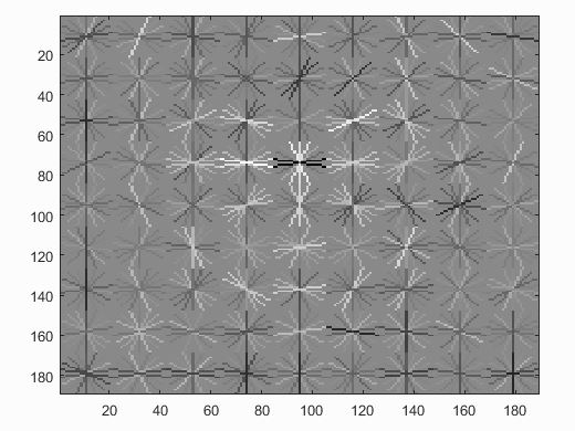 Cell size = 4
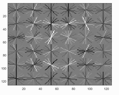 Cell Size = 6
|
As the cell size reduces, greater percision can be observed, but at the cost of computational time. When we squint our eyes a bit to observe closely, the cell size of 4 looks closer to a face compared to the HoG visualization of cell size of 6.
Results with and without hard negative mining
| Precision Recall curve for baseline implementation |
|
|
To conclude, the major factors affecting the accuracy here are the sampling of positive HOG feature, with mirrored results, the number of negative HOG features, the lambda value of SVM training(to an extent), multi-scale sliding window and mining hard negative can help to the accuracy.