Project 5: Face Detection with a Sliding Window
Face detection pipeline based on the sliding window detector of Dalal and Triggs 2005.
Given a training data set and testing data set, the detection pipeline:
- Converts the positive and negative training images to feature vectors.
- Trains a linear SVM classifier on the training data.
- Mines additional "hard negative" training examples.
- Re-trains a linear SVM classifier using the augmented data set.
- Runs the detector on the test data set.
- Visualizes detected faces and reports testing accuracy.
Positive Training Examples
The positive training examples are the 6,713 cropped 36×36 faces from the Caltech Web Faces project. To augment the positive training examples, each image is "jittered" with three transformations (Tmirror , TrotL , and TrotR ) for a total of (6,713 × 4) = 26,852 examples total. Some qualitative results of these transformations are shown in figure 1 below. After augmenting the set of positive training images, each image is converted to a Histogram of Gradients (HoG) template and reshaped as a feature vector. The dimensionality of the feature space is determined by the HoG parameters.
Original image I |
Mirrored image Tmirror(I) |
Left-rotated image TrotL(I) |
Right-rotated image TrotR(I) |
 |
 |
 |
 |
 |
 |
 |
 |
Figure 1. "Jittering" images to augment the training data set.
The transformation Tmirror reflects the input image horizontally. The transformations TrotL and TrotR rotate the image by θ=10 degrees counterclockwise and clockwise (respectively). Note that the input image is first padded (symmetrically) to fill in empty regions when rotating. Jittering the positive examples (while holding other parameters constant) increased average precision from ~83% to ~85%.
Negative Training Examples
The negative training examples are sampled from a database of 275 non-face images from Wu et al. and the SUN scene database. The examples are collected by randomly cropping a specified number of 36×36 patches (same size as positive examples) from each non-face image. Each cropped image is then converted to a HoG template and reshaped as a feature vector.
 |
 |
 |
 |
 |
Figure 2. Randomly-cropped negative training examples. |
||||
Classifier Training
The positive and negative training examples are used to train a linear SVM classifier (vl_svmtrain). Figure 3 below shows the learned face template for several different HoG cell sizes. Figures 4 and 5 shows initial classifier performance on the training data set when using ~10,000 negative examples, HoG cell size 6, and SVM regularization parameter 0.001.
|
|
|
|
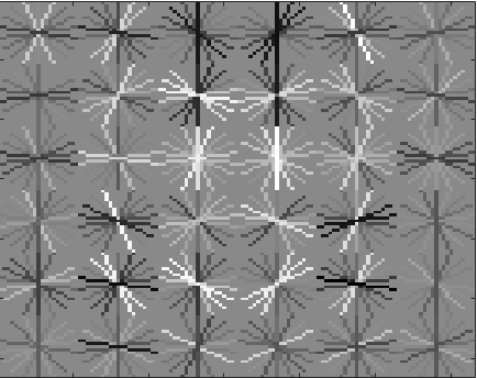
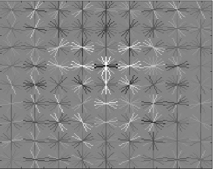
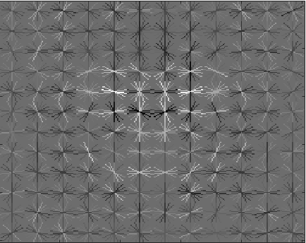
Figure 3. Visualization of HoG template learned from the training examples using cell sizes 6, 4, and 3 (from left to right). The template visibly captures the shape of head and shoulders. Using a smaller cell size increases the feature dimensionality and requires more computation time when training and testing. |
||
 |
||
|
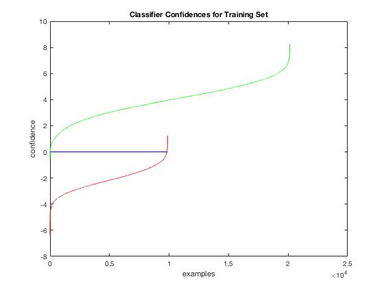
Figure 4. Classifier confidences for positive training examples (in green) and negative training examples (in red). The classification boundary (in blue) is at 0 by default, however the threshold is lowered at test time. Ideally, all of the red line should be below the boundary and all of the green line should be above the boundary. |
||
Training accuracy |
True positive rate |
False positive rate |
True negative rate |
False negative rate |
| 0.997 | 0.670 | 0.003 | 0.326 | 0.001 |
Figure 5. Initial training accuracy for the face detector.
Hard Negative Mining
To improve detection accuracy, the initial trained classifier is run on the negative training images to find examples incorrectly classified as positives (i.e. negative examples that are "hard" to classify correctly). The size of the training data set is kept constant by replacing easier negatives with harder negatives. Figure 6 below shows some examples of hard negatives. Figures 7 and 8 show detector performance when using ~5,000 negative examples. The hard negatives were detected at a single scale, using a window step size of 5 and detection threshold -0.5.
 |
 |
 |
 |
 |
Figure 6. Some hard negative examples. The initial classifier labeled these as faces with confidence > 1. |
||||
 |
 |
|
Figure 7. (Left) classifier confidences after training on 5000 random negative examples. (Right) classifier confidences after mining 203 harder negatives. Note that some negative examples are now above the classification boundary. |
|
Testing accuracy |
Training accuracy |
True positive rate |
False positive rate |
True negative rate |
False negative rate |
|
| without mining | 0.825 | 0.992 | 0.837 | 0.000 | 0.155 | 0.008 |
| with mining | 0.848 | 0.996 | 0.841 | 0.001 | 0.154 | 0.003 |
Figure 8. Mining hard negatives to curate a training set of fixed size (5000 examples).
Although mining hard negatives shows small accuracy improvements for training sets of fixed size (as shown in figure 8 above), greater performance gains were observed when using an increased number of random negatives in the initial training set. Mining hard negatives is expensive, so this step was not used at test time.
Test Performance
The CMU+MIT data set (the most common benchmark for face detection) was used to test accuracy of the face detection pipeline. This test set contains 130 images with 511 faces. The figures below show the pipeline's performance on the test set when using: ~100,000 negative examples (without mining), SVM regularization parameter 0.001, HoG cell size 3, scale step size of 0.8, minimum scale of 0.1, and a window step size of 1.
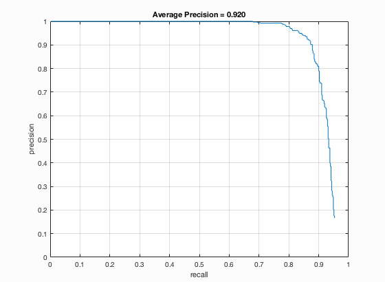
Figure 9. Precision-recall curve for the test set when using classification threshold -0.5.
|
|
|
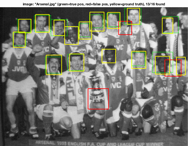
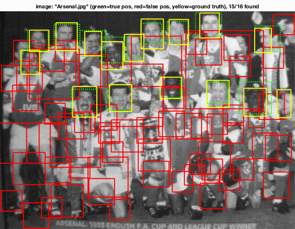
Figure 10. Example of detections on the test set. (Left) using a detection threshold of 1.0 yields few false positives. (Right) lowering the threshold to -0.5 increases recall at the cost of reduced precision. |
|
Additional Test Cases
The detection pipeline was also tested on the provided class photos. Ground truth bounding boxes are not included for these images, however qualitative results can be seen in the figures below. The detection threshold was increased to 1.0 for these test images.
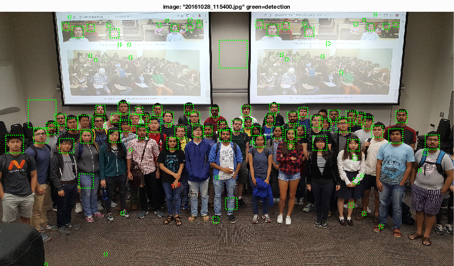
Figure 11. Detections for "easy" test case (neutral, frontal faces).
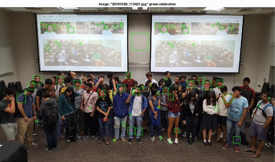
Figure 12. Detections for "hard" test case (intentional obfuscation).