Project 5 / Face Detection with a Sliding Window
Part 1: Train the Classifier
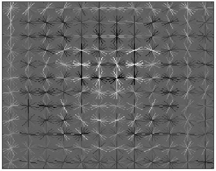
Training the classifier had three steps - finding positive examples, finding negative examples, and creating the classifier. Finding the positive examples was mostly done for us, all I had to do was open the images and creat HoGs for each ground truth face. Additionally, I added a mirror image of each face to increase the training size. This allowed the learned detector to be mostly symmetrical. The negative examples were slightly more involved. I had to extract the windows randomly from the image set. This could've been done on multiple scales to increase precision, but I got good results without doing so, so I left it on a single scale. Finally, training labels were added to the data and an SVM was trained. I used the suggested lambda value of .0001, which worked well. The image below shows the learned detector when run with a cell size of 3 pixels. I thought it was very interesting to see that a face can (kind of) be seen in the detector.
Part 2: Implement the Sliding Window Detector
The next step was to use the detector in a sliding window to find faces without ground truths. To do this, the HoG was computed for the entire image, and then each possible window was extracted and tested to see if it contained a face - this was possible because the SVM does not take long to classify, so it was able to run relatively quickly even while iterating over the entire image. To account for different sizes of faces, this process was repeated on multiple scales.
Once implemented, there were a few parameters to be tuned. First was how much to reduce the scale at each step. This created a tradeoff between run time and accuracy. I settled on reducing the size of the image by .9 each time, until it was too small. This yielded acceptabe precisions and run times. Next was the confidence threshold. This parameter created a tradeoff between precision and number of false positives. I ended going with .8 for most iterations. There were still many false positives, but the precision was good. Finally, the cell size parameter could be tweaked. Again, this was a trade off between run time and accuracy. I used the sizes of 3, 4, and 6. Results are listed below.
Results
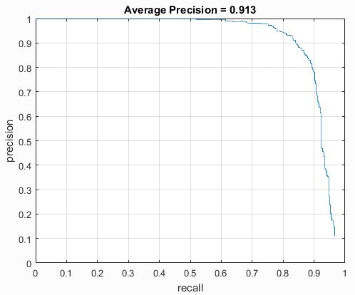
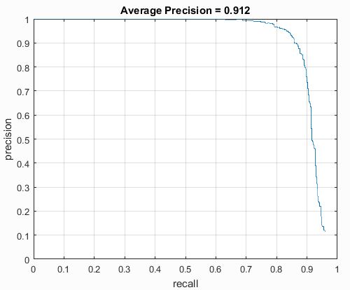
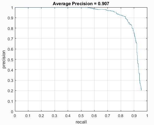
I ran trials with different cell sizes to see the effect on precision. With a cell size of 3, the precison was .913. With a cell size of 4, the precision was .912. With a cell size of 6, the precision was .907. I'm not entirely sure why the precisions were higher than the baseline listed in the project, but I think that it is most likely because I used many scales for each image. The precision-recall curves are shown below.
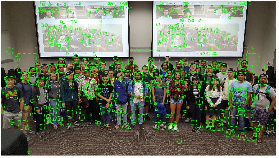
I also ran the detector on the class images, just to see how they turned out. There were a distracting number of false positives, but it still seemed to detect most of the faces. By my inspection, it appears to have detected all of the faces of the actual people in the class (with the exception of the guy who tilted his head and a few obscured people), and it even did well on the projected images in the back.
In conclusion, I found this project very interesting. I really like seeing the intersections of machine learning and computer vision. Especially in this case, when a bunch of straight forward concepts (classifiers, HoGs, etc.) can be put together to do a seemingly complicated task.