Project 5 / Face Detection with a Sliding Window
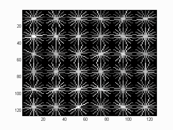
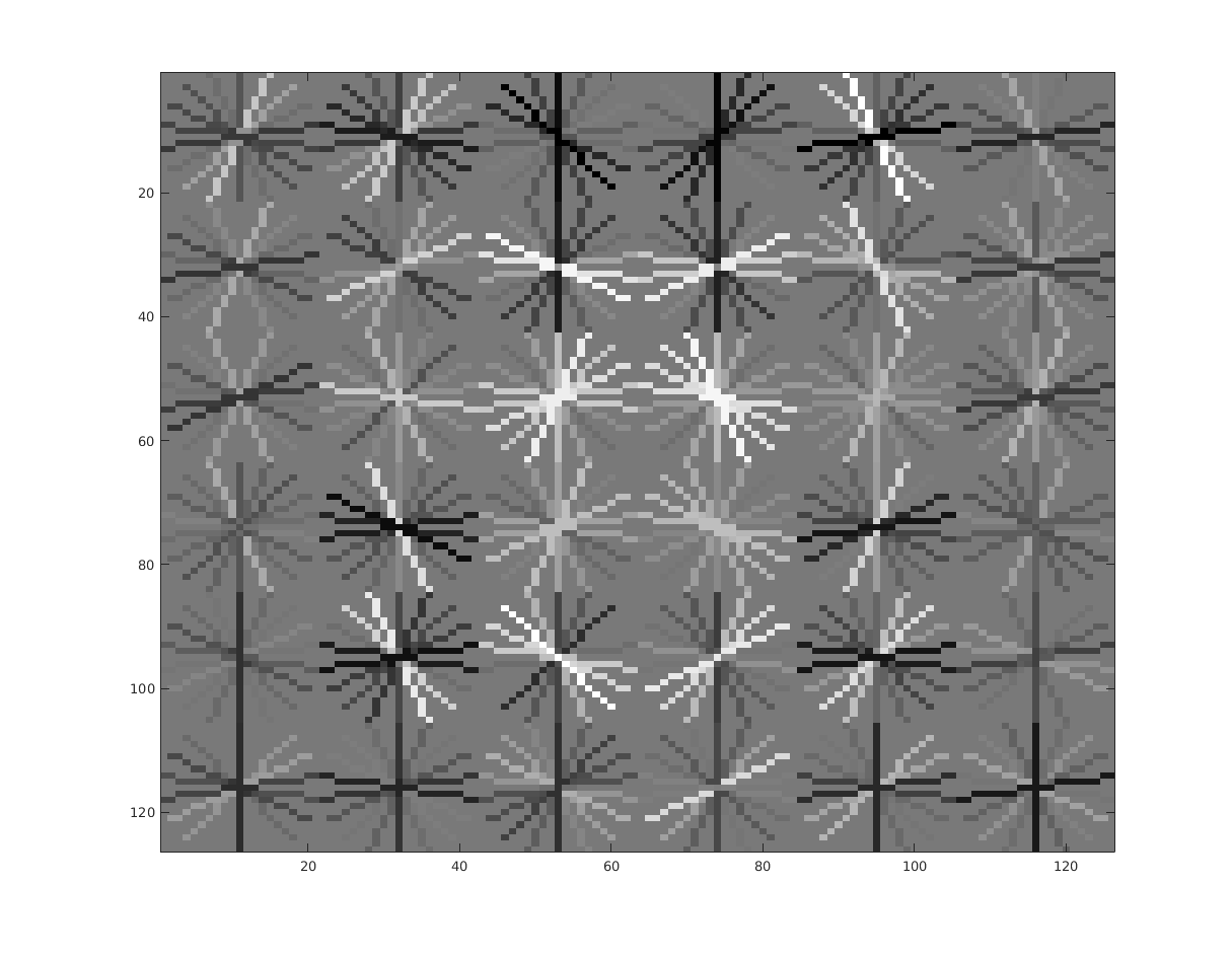
Example of a HoG descriptor.
The sliding window model is conceptually simple: independently classify all image patches as being object or non-object. Sliding window classification is the dominant paradigm in object detection and for one object category in particular -- faces -- it is one of the most noticeable successes of computer vision. For example, modern cameras and photo organization tools have prominent face detection capabilities. These success of face detection (and object detection in general) can be traced back to influential works such as Rowley et al. 1998 and Viola-Jones 2001. You can look at these papers for suggestions on how to implement your detector. However, for this project the author will be implementing the simpler (but still very effective!) sliding window detector of Dalal and Triggs 2005. Dalal-Triggs focuses on representation more than learning and introduces the SIFT-like Histogram of Gradients (HoG) representation (pictured to the right). The author will not implement HoG because the project 2 was very similar work: implementation of the SIFT. The author will be responsible for the rest of the detection pipeline, though -- handling heterogeneous training and testing data, training a linear classifier (a HoG template), and using his classifier to classify millions of sliding windows at multiple scales. Fortunately, linear classifiers are compact, fast to train, and fast to execute. A linear SVM can also be trained on large amounts of data, including mined hard negatives. This report has the following main sections:
- Obtain positive features,
- Obtain negative features,
- Build classifier via SVM from positive and negative features,
- Detection via sliding window,
- Implement a HoG descriptor (Extra credit), and
- Results
Obtain positive features
The Caltech Web Faces project provide us with 6713 cropped faces, and this is the positive images the author uses. They are all cropped and resized to 36x36 grayscaled images. All we have to do is compute the histgram of oriented gradients (HoG) and vectorize each feature to a row vector. The corresponding function lives in get_positive_features.m. The key part of this code looks like the below:
% obtain positive features
features_pos = zeros(num_images, (template_size / cell_size)^2 * 31);
for i = 1:num_images
    filename = sprintf('%s/%s', train_path_pos, image_files(i).name);
    im = single(imread(filename));
    hog_feature = vl_hog(im, cell_size);
    features_pos(i, :) = reshape(hog_feature, [1 size(features_pos, 2)]);
end
Obtain negative features
The negative images here are from Wu et al. and the SUN scene database. Basically, any images that do not contain a face work as a negative image. We want as many negative images as the order of 10^4 ~ 10^6. Since we only have approximately 300 negative images, we need to crop part of the image and use it as one negative feature. In other words, more than one features are extracted from one image. Negative images are all bigger than 36x36. In the algorithms of the authors, the number of negative features extracted from one image is computed based on the necessary number of the negative features. Then, the region of interest is randomly picked, the HoG of the region is calculated. The procedure is repeated until the number of the negative features reaches to the goal number. The same procedure is repeated at multiple scale of the negative image. The following code achieves this:
% obtain negative features
for i = 1:num_images
    filename = sprintf('%s/%s', non_face_scn_path, image_files(i).name);
    imlarge = imread(filename);
    scale = [1 0.9 0.8];
    per_img_features = [];
    for s = 1:size(scale, 2)
        im = single(imresize(imlarge, scale(s)));
        while(size(per_img_features, 1) < ceil(sample_per_image/size(scale, 2)) * s)
            rect = [randi(size(im, 2) - template_size - 1),... % note col
                    randi(size(im, 1) - template_size - 1),...
                    template_size, ...
                    template_size];
            roi = imcrop(im, rect);
            hog_feature = vl_hog(roi, cell_size);
            per_img_features = [per_img_features; reshape(hog_feature, [1 (template_size/cell_size)^2 * 31])];
        end
    end
    tmp_features = [tmp_features; per_img_features];
end
rand_ind = randperm(size(tmp_features, 1));
features_neg = tmp_features(rand_ind(1:num_samples), :);
Build classifier via SVM from positive and negative features
Building a classifier is very simple using thevl_svntrain. All the positive features are labeled one, and everything else is negated. This operation is done inside proj5.m. You need to tune the lambda to make the classifier best perform.
% build a classifier via SVM
Y = [ones(1, size(features_pos, 1)), -1 * ones(1, num_negative_examples)];
lambda = 0.01;
[w, b] = vl_svmtrain(X', Y, lambda);
Detection via sliding window
The idea of the sliding window is straightforward. The small section of the source image is compared to some kind of a template. The template is typically smaller than the source image in any dimension, and the corresponding small section of the source image is the same dimension as the template's. For example, when faces are searched over a 400x400 source image, a 40x40 face template is searched over the source image from left to right, and from top to bottom by sliding the template over the entire source image. Here, the template is a 36x36 HoG feature, and the SVM model is used to compare the template and a corresponding section of the source image. All the location whose confidence is beyond a threshold are stored, and the non-maximum suppression makes the final outputs. Since we don't know how much of the pixels of the source image is filled by a face, the above operation is done by scaling the source image by many different scales. Ideally, the window should be shifted one pixel by one pixel, but you can increase the step size. This significantly sppeds up the process but does not critically hurt the results. The codes are shown below:
% sliding window algorithm
for s = 1:size(scale, 2)
    im_scaled = imresize(img, scale(s));
    max_col = size(im_scaled, 2) - template_size + 1;
    max_row = size(im_scaled, 1) - template_size + 1;
    for col = 1:step_size:max_col
        for row = 1:step_size:max_row
            roi_rect = [col, row, template_size, template_size];
            roi = imcrop(im_scaled, roi_rect);
            hog_feature = vl_hog(roi, cell_size);
            feature_of_this_window = reshape(hog_feature, [1 (template_size/cell_size)^2 * 31]);
            confidence = feature_of_this_window * w + b;
            if(confidence > confidence_threshold)
                cur_confidences(end+1, 1) = confidence;
                cur_bboxes(end+1, :) = 1.0/scale(s)*[col, row, col + template_size - 1, row + template_size - 1];
                cur_image_ids(end+1, 1) = {test_scenes(i).name};
            end
        end
    end
end
[is_maximum] = non_max_supr_bbox(cur_bboxes, cur_confidences,...
    size(img));


cur_confidences = cur_confidences(is_maximum, :);
cur_bboxes      = cur_bboxes(is_maximum, :);
cur_image_ids   = cur_image_ids(is_maximum, :);

bboxes      = [bboxes;      cur_bboxes];
confidences = [confidences; cur_confidences];
image_ids   = [image_ids;   cur_image_ids];
Implement a HoG descriptor (Extra credit, up to 10 pts)
In this section, the author replicates the function equivalent to the vl_hog in the vl_feat library. The vl_feat is a powerful and optimized library in image processing, and the purpose of this section is not to overcome the performance of the vl_feat but to let the author understand the mechanism of the HoG.
The procedure to compute a HoG feature is as follows. First, an image is separated into many cell_size by cell_size images. The gradients in x and y directions are computed, and the angles and magnitudes of the gradients are stored as a histogram of the orientations; thus, the number of the bins of the histgram is the number of the orientations to which the gradient vectors are projected. In this implementation, the number of bins is 8, and the cell size is 6. This operation is very similar to the one done in the SIFT, but the main difference is that the Hog features evaluated densely, not sparsely. The SIFT features are only evaluated at interest point extracted by the corner Harris algorithm or any kind of a similar method, but the HoG features are evaluated a regular overlapping grid. Then, the HoG features are normalized over the cell. The below code extracts the HoG descriptor.
function hog_feature = my_hog(im, cell_size, orientations_number)
    [H, W] = size(im);
    orientation_num = orientations_number;
    max_col = floor(W / cell_size);
    max_row = floor(H / cell_size);
    g_deriv_x = fspecial('sobel');
    g_deriv_y = g_deriv_x';
    Ix = imfilter(im, g_deriv_x);
    Iy = imfilter(im, g_deriv_y);
    orientations = zeros(max_col, max_row, cell_size, cell_size);
    mags = zeros(max_col, max_row, cell_size, cell_size);
    w = cell_size;
    h = cell_size;
    falloff_sigma = 3 * w;
    g_falloff = fspecial('Gaussian', [w h], falloff_sigma);
    for l = 1:max_col
        x = cell_size * (l - 1) + 1;
        for k = 1:max_row
            y = cell_size * (k - 1) + 1;
            for j = 0:w-1
                for i = 0:h-1
                    x_fd = Ix(y + i, x + j); % x first derivative
                    y_fd = Iy(y + i, x + j); % y first derivative
                    orientation = floor(atan2(y_fd, x_fd) / (2 * pi / orientation_num)) + floor(orientation_num / 2);
                    orientations(l, k, i + 1, j + 1) = orientation;
                    mag = sqrt(abs(y_fd)^2 + abs(x_fd)^2);
                    mags(l, k, i + 1, j + 1) = mag;
                end
            end
            gaussian_mag = squeeze(mags(l, k, :, :)) * g_falloff;
            mags(l, k, :, :) = gaussian_mag;
        end
    end

    hog = zeros(max_col, max_row, orientation_num);
    for l = 1:max_col
        for k = 1:max_row
            sum_of_this_cell = 0;
            for j = 1:w
                for i = 1:h
                    for ori = 0:orientation_num - 1
                        if(ori == orientations(l, k, i, j))
                            hog(l, k, ori + 1) = hog(l, k, ori + 1) + mags(l, k, i, j);
                            if(isfinite(mags(l, k, i, j)))
                                sum_of_this_cell = sum_of_this_cell + mags(l, k, i, j);
                            else
                                disp('not finite!');
                            end
                        end
                    end
                end
            end
            hog(l, k, :) = hog(l, k, :) / sum_of_this_cell;
        end
    end
    hog_feature = reshape(hog, [1 max_col * max_row * orientation_num]);
end
Results
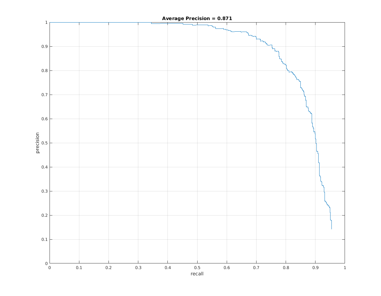
First of all, let us show the results of the classifier. 10000 negative images are used to train the classifier, and the lambda = 0.001.
|
| Evaluation of the classifier |
| accuracy | 0.997 |
| false positive rate | 0.002 |
| true negative rate | 0.596 |
| false negative rate | 0.001 |
|
| Precision vs recall. |
|
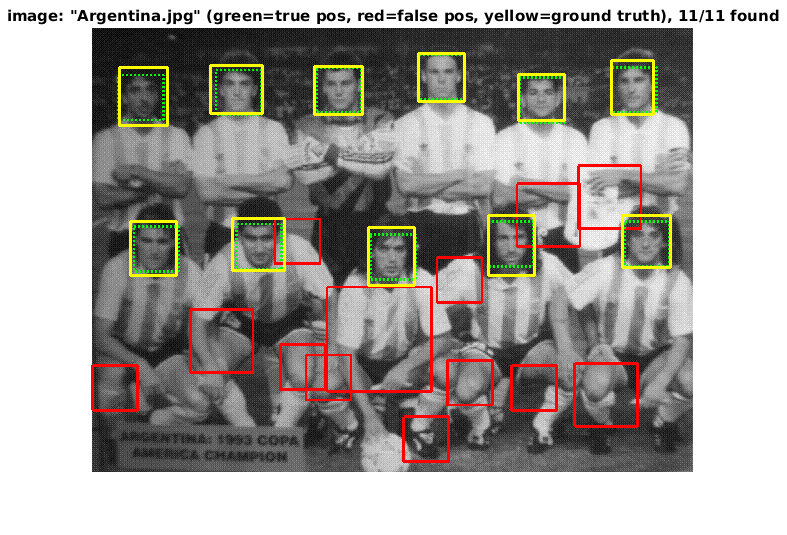
| Example of face detection |
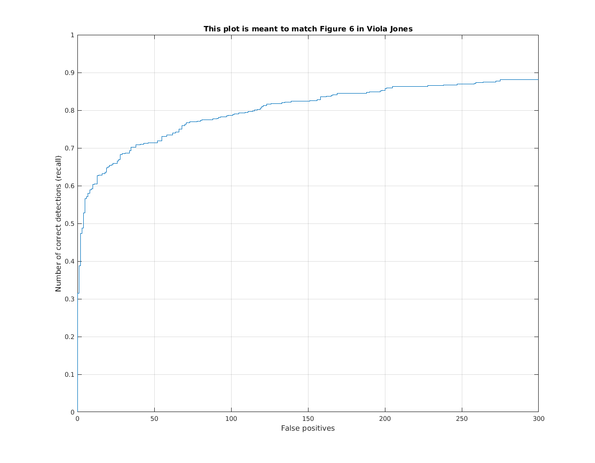 | 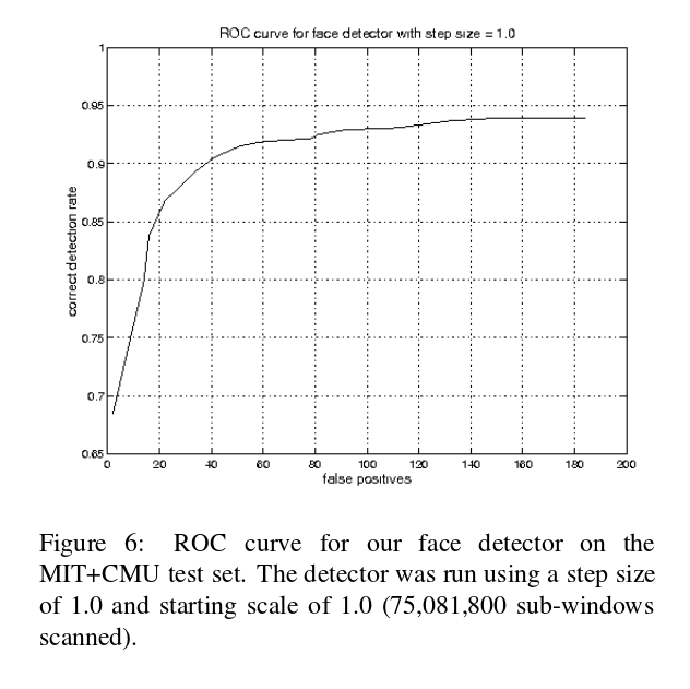 |
| The author's results | From Viola Jones paper |