Wengling Chen

Basic Implementation

Get Positive/Negative Features

The positive samples are pre-cropped 36x36 black and white small images of different faces, and there are altogether around 7000 of them.
The way I got my negative samples are randomly cut 36x36 patches from all non-face images provided. For simplicity, I did not do multi-scale sampling at this stage, and the result I got is still ok.
After I got the samples, I just use the vl_hog function to extract HoG features from each sample. The parameter cell_size is critical: generally speaking, the smaller the cell size, the finer details extracted features will have, but obviously it will be a lot slower. The default cell size is 6, and for my best result, I use a cell size of 2 which cause the program to run for a really long time. Also, the number of negative samples can be adjusted. I only used 50K samples, and I think that is basically enough because the linear classifier is unlikely to benefit more from more negative samples.

Linear SVM

There is not much to say about linear SVM. The only parameter to tune is the lambda, which in this case, I just randomly tried some values like 0.01, 0.001, 0.0005 and so on. It seems like as long as lambda is in this range, there is not a big difference between resulting accuracies.

Multi-scale sliding windows detector

The multi-scale sliding windows detector basically has two important properties, as its name shows: it detects at multiple scales, and it uses sliding window. In practice, I found that using proper scales are very important, even more important than tuning the SVM. After several tries, I soon found that many of the images in the test set has very large faces, so I biased my scaling factor toward smaller numbers so that the detector will easily catch more larger faces, and it works pretty well (although it is actually overfitting). Also, the more levels your detector detects on, the higher the resulting accuracy will be. Another thing to adjust is the threshold of rejecting proposed bounding boxes. However, I actually set it to very low value in order to get higher accuracy (and of cause a lot of false positives).

Accuracy/Performance Report

The first table shows accuracies under different parameters, as well as the resulting HoG template images. Parameters are listed in the table.

Parameters	Precision curve	Recall v. False Positive	HoG template
cell_size=6;lambda=0.01;threshod = -1;1 scale
cell_size=2;lambda=0.001;threshod = -0.5;9 scales

Here I am going to discuss a little about the results. The first run, which is obvious not very good, misses many faces. However, in some simple scenes it is actually working well. See image 1 in the table. Image 2 shows it can actually detect a blurred face. Image 3 shows it can also detect some artificial faces. To my surprise, it actually find all faces in image 4:

Image 1	Image 2
Image 3	Image 4

For the second run, the precision is much higher. However, this is actually done at the cost of very large number of false positives. In image 1, you can see that it is almost flooded with false positives, and somehow it still missed one face. In Image 2, it detected this artificial face. The HoG template with cell size 2 explains what happened in Image 3: look at that HoG template, doesn't it look like a front face? And the face the detector missed in Image 3 is actually a side face--which is hard for this HoG+SVM, but with a CNN, it is quite easy(see later parts). Image 4 shows the affect of multi-scale: it detected this large face.

Image 1	Image 2
Image 3	Image 4

Extra Credits: Find and utilize alternative positive training data/Use additional classification schemes

Overview

I put this two together, because in my case, they are closely related. The idea of deep learning, which is backed up by the huge amount of data we produce every day, has just changed the whole academia and industry. Now, convolutional neural networks, or CNNs, are almost a must-have in computer vision area, as well as many related fields. Here I just want to try out the power of modern CNNs, and I decide to train my own model and see its performance on the provided test set.

The network I used: Faster R-CNN[1]

This is one of the state-of-the-art object detection networks. It is developed from their original work of Fast R-CNN. Although its original intention is to be a network that can propose and classify objects really fast(up to 5fps), here I just used its ability to detect certain classes of objects. It actually works very well, with an mAP of 75.9 on PASCAL VOC 2012 test set. I will not go down into the details of this network because that is in authors' report.(See references)
There are two underlying networks they implemented: ZF[2] and VGG-16[3]. I used the latter one, because its performance is slightly better.

The datasets I used: Caltech 10,000 Web Faces[4] and WIDER FACE: A Face Detection Benchmark[5]

To efficiently train a good deep neural network, a large number of training samples is indispensable. The Caltech Web Faces, which is actually what we used for positive examples, are quite good training data. I used the original dataset of whole images with colors, not the cropped versions provided. The problem of that set is, it does not have bounding boxes as ground truth. Instead, they give positions of eyes, mouths and noses. Luckily, Prof. Hays wrote some code to convert them into bounding boxes, and I just took that.
The second set, WIDER FACE, has much more sample with various kinds of gestures, positions and in different environment. It is really a good set, I would say, and they give ground truth to us. When I mixed these two datasets together, basically I got a training+validation set of over 17,100 images, and also several thousand test images. That is definitely a big number for single machine training.

Training

Training of this network is hard: not only because this is the first time I try to train a deep neural network, but also because it is extremely slow. Even with the help of a GPU, it took me over 7 hours to finish training one model--and the model is not fine tuned. There are several things I can change, and basically one of the most important thing is the learning rate. I could not try many times, so I just used some moderate value, and I got some OK results.
One interesting observation: I think the saying that more data is better is true. Using the WIDER set proved to be better than only using Caltech set, and using both was even better.

Performances

Here I am going to show a table comparing the three models I trained. The first one is trained only on Caltech set, the second one is trained only on WIDER set, and the third one is trained on both sets. It should be noted that I used different parameters when training the three models, as shown in the table. Meanwhile, when I was training the first model, I happened to make some mistakes on the metadata of training images, so its actual performance should be better than shown here.
Also notice that the parameters used when classifying faces will also affect performance, as shown in table 2.
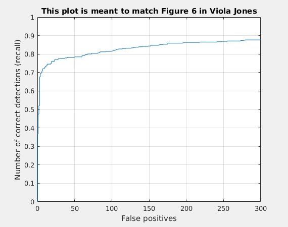
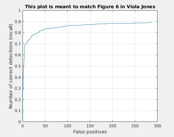
From the graphs we can see there is some huge improvements by using this R-CNN. The first thing that gets my attention is, the number of false positives is extremely low comparing to the HoG+SVM method. When I got 89% precision on HoG+SVM, I actually produced over 47K false positives. Here, there are only 50~290, which is really a small number.

The highest AP I achieved is 0.956, as shown in table 2.

Table 1:

Trained on	Parameters	Precision curve	Recall v. False Positive
Caltech Webfaces	base_lr=0.00001;stepsize=30000;num_iter=70000;iter_size=2
WIDER	base_lr=0.0001;stepsize=30000;num_iter=70000;iter_size=2
Caltech Webfaces + WIDER	base_lr=0.001;stepsize=30000;num_iter=100000;iter_size=2

Table 2, both are the third model:

Classify Parameters	Precision curve	Recall v. False Positive
Pre-scaled;Confidence_thres = 0.001;nms_thres = 1
Confidence_thres = 0.7;nms_thres = 0.3

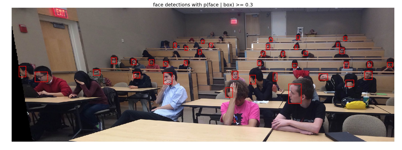
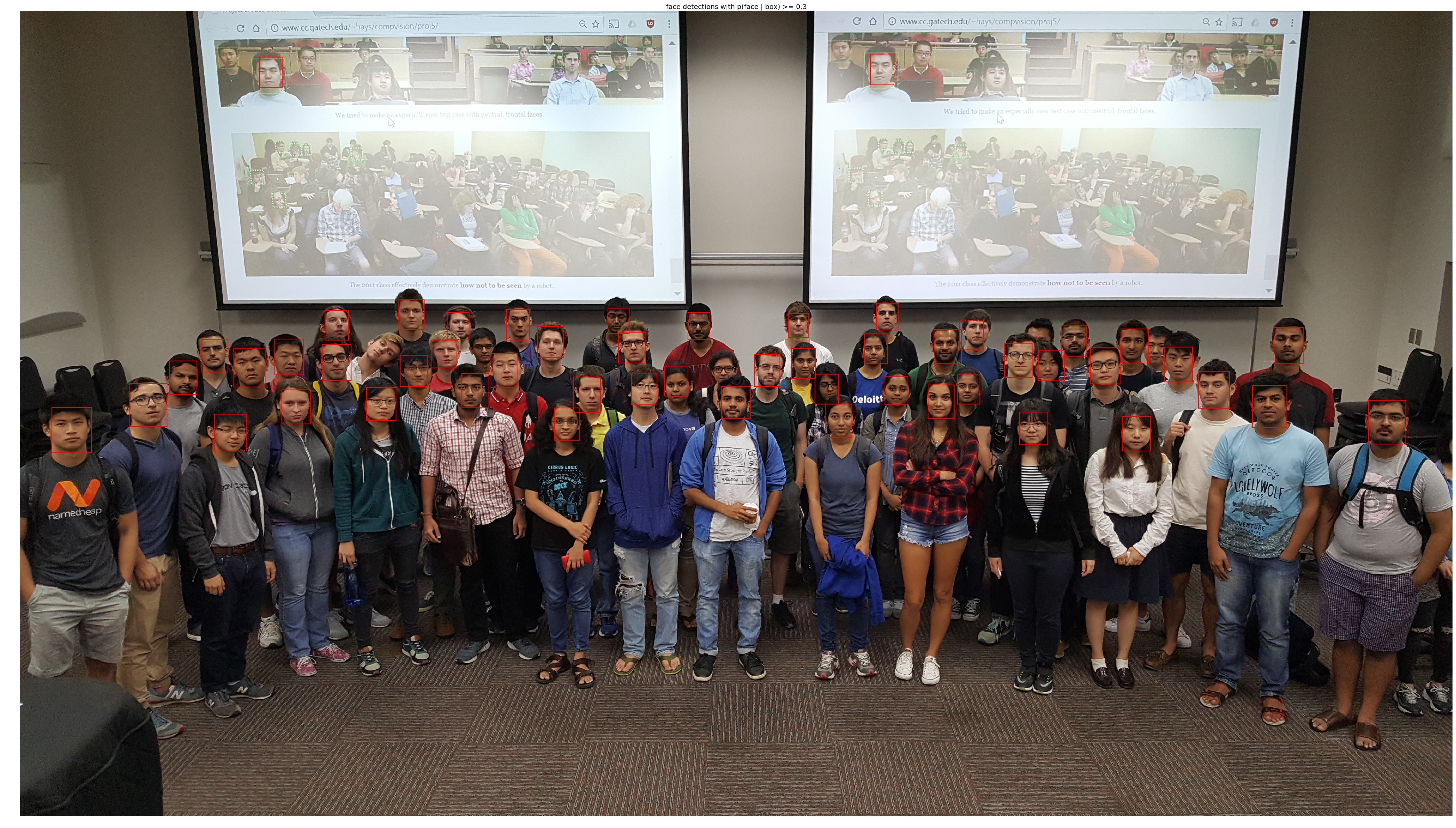
Performance on extra test scenes. It is brilliant!

With the third model I trained on both sets and some tuning on parameters, I got very good results on the extra test scenes. I think these results are really amazing. Actually, the network is very good at detecting 'anomalous' faces such as side faces and partially covered faces. Have a look at those results!

Something interesting: it seems that Prof. Hays' face can be easily detected under most parameters.

References

[1] Ren, Shaoqing, et al. "Faster R-CNN: Towards real-time object detection with region proposal networks." Advances in neural information processing systems. 2015.
[2] Zeiler, Matthew D., and Rob Fergus. "Visualizing and understanding convolutional networks." European Conference on Computer Vision. Springer International Publishing, 2014.
[3] Simonyan, Karen, and Andrew Zisserman. "Very deep convolutional networks for large-scale image recognition." arXiv preprint arXiv:1409.1556 (2014).
[4] Caltech 10, 000 Web Faces http://www.vision.caltech.edu/Image_Datasets/Caltech_10K_WebFaces/
[5] Yang, Shuo and Luo, Ping and Loy, Chen Change and Tang, Xiaoou. "WIDER FACE: A Face Detection Benchmark" IEEE Conference on Computer Vision and Pattern Recognition. 2015