Xiaoxi Han

1. Handing training data

The training data is consisted of two parts: images with face and images without face. Even though all the positive images (with face) are configured properly as they are of same size and the face size are approximately the same, the negative images are of different sizes and scales. Therefore, to achieve better performance, I used a scale factor of 0.9 when getting HoG features from negative images, meaning that I scale the image down to 0.9*original scale recursively and get some new features until the image is too small to achieve new features. I used 10000 negative images to get the features. Even though more image will improve the performance, it will take much longer to train, thus I kept using 10000 negative images.

2. Training classifier

This part is pretty strait forward, and there is one parameter lambda to tune with. After trying different lambda (0.1, 0.001 and 0.0001), the smallest worked the best, so I chose 0.0001.

3. Sliding window detection

In this part, I used multiple scale with 0.9 as the scale factor. I have also tried 0.7, but the average accuracy dropped by arround 6%, so the larger the scale factor is, the better the performance will be. However, the run time grows significantly when the scale factor becomes larger. When scale factor is 0.7 and step size is 6, the entire pipeline runs in less than a minute, whereas when scale factor is 0.9 and step size is 6, the run time is approximately 3 minutes.
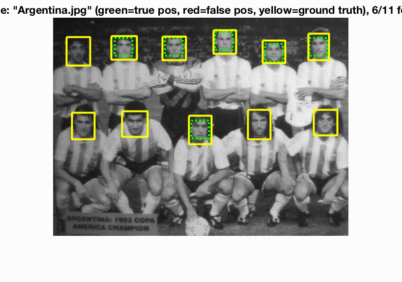
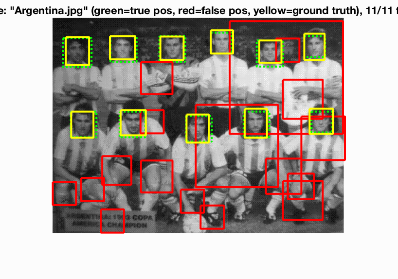
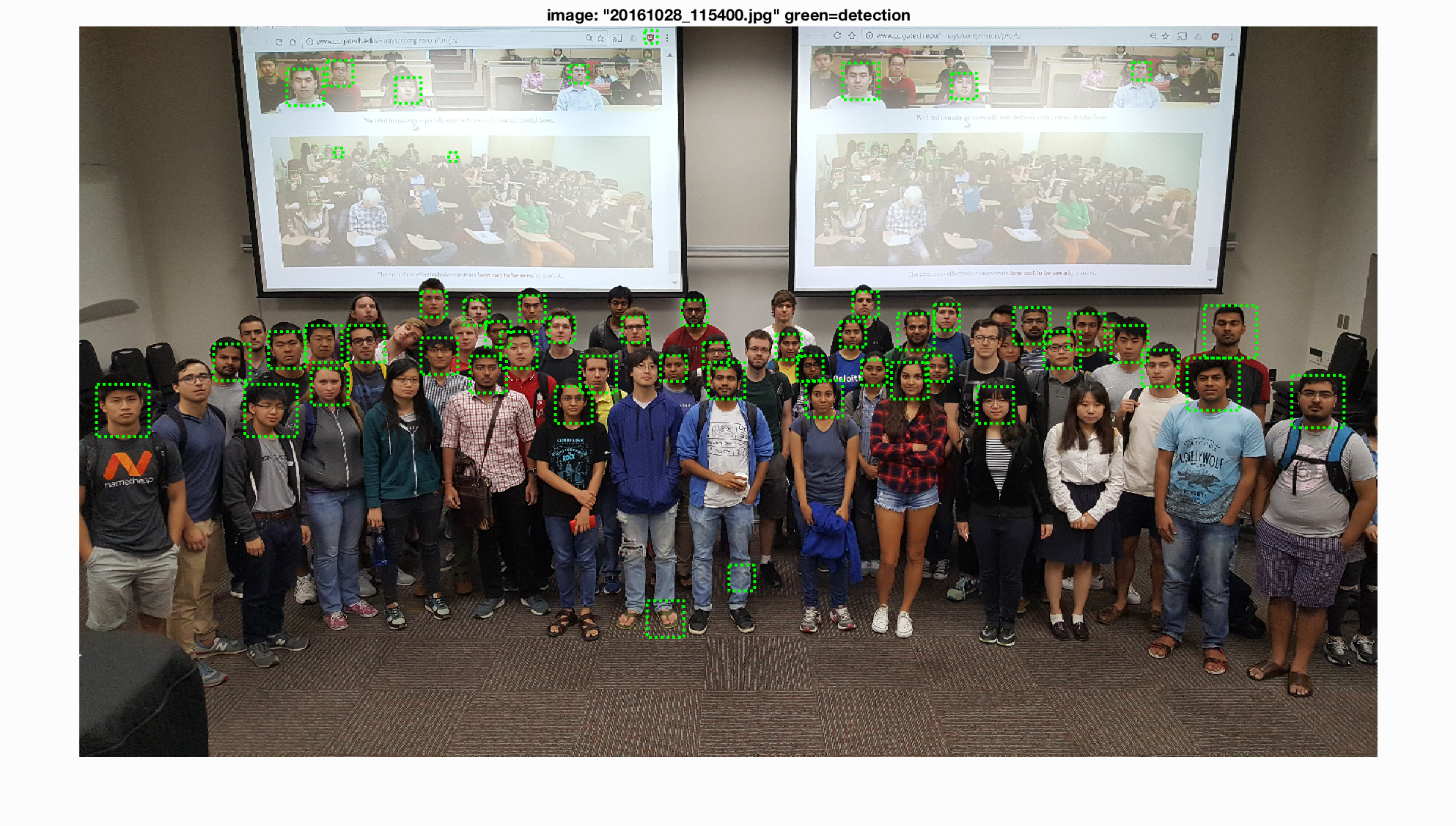
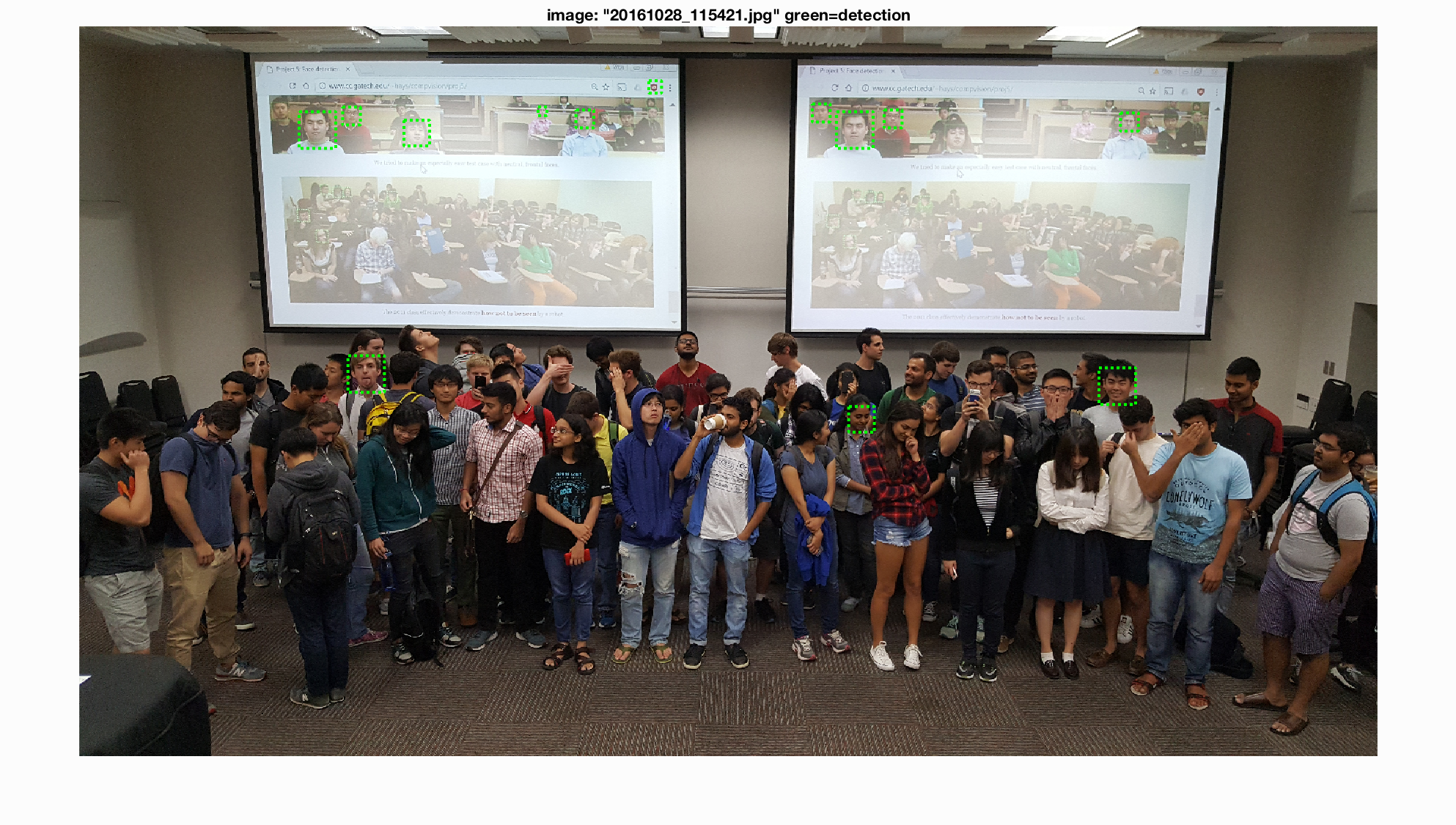
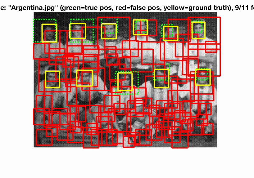
Another factor that I have modified is the confidence threshold. When the treshold gets smaller, the accuracy gets higher, however the false positive rate gets higher too. To achieve better accuracy, I set the threshold to 0.7 when measuring the highest accuracy, whereas in the class image listed at the bottom of the page, since I want to detect the face with fewer false positive, I set the threshold to 0.3.
The step size also affacts run time significantly. When the step size is smaller, the pipline runs much slower. When I set step size to 4, the total runtime is 8 minutes, and when the setp size is 3, the runtime is 14.5 minutes.
The performance of the algorithm with different step size and fixed scale factor (0.9) is shown below. Normally when step size is smaller, the accuracy gets much better.

Results in a table

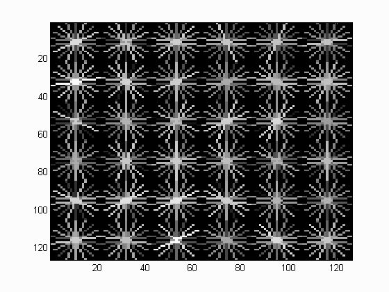
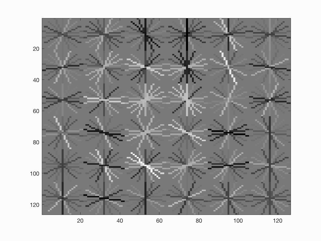
Face template HoG visualization for the starter code. This is completely random, but it should actually look like a face once you train a reasonable classifier.

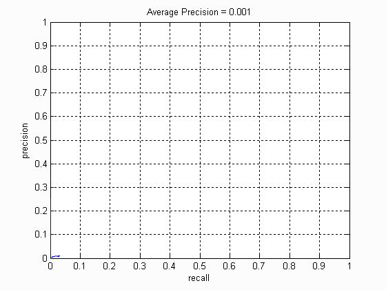
Precision Recall curve for the starter code.

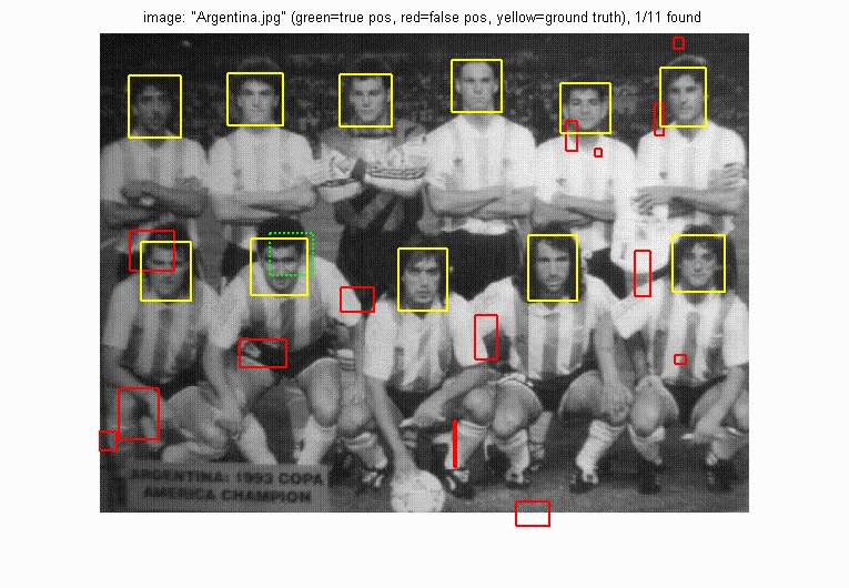
Example of detection on the test set from the starter code.

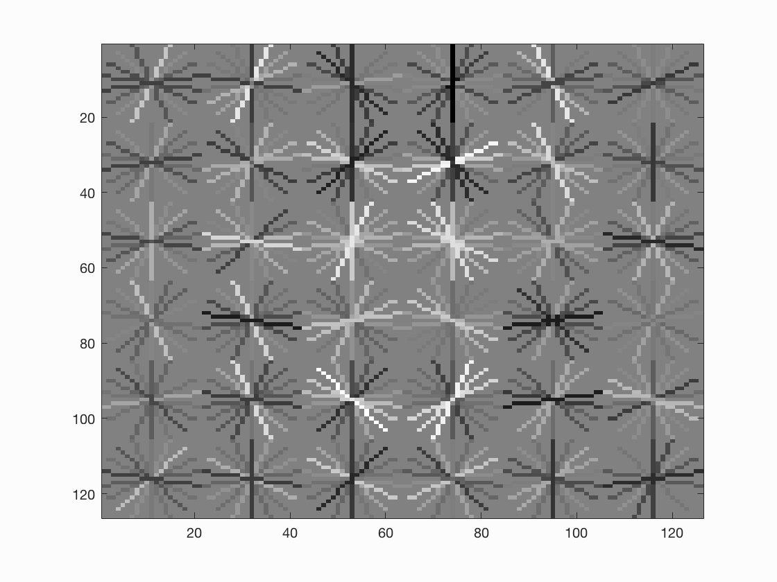
Face template HoG visualization with single scale, threshold = 0.7, step size = 6. We can see that the HoG visualization starts to look like a face with a round circle.

Precision Recall curve for the starter code.

Example of detection on the test set from the starter code.

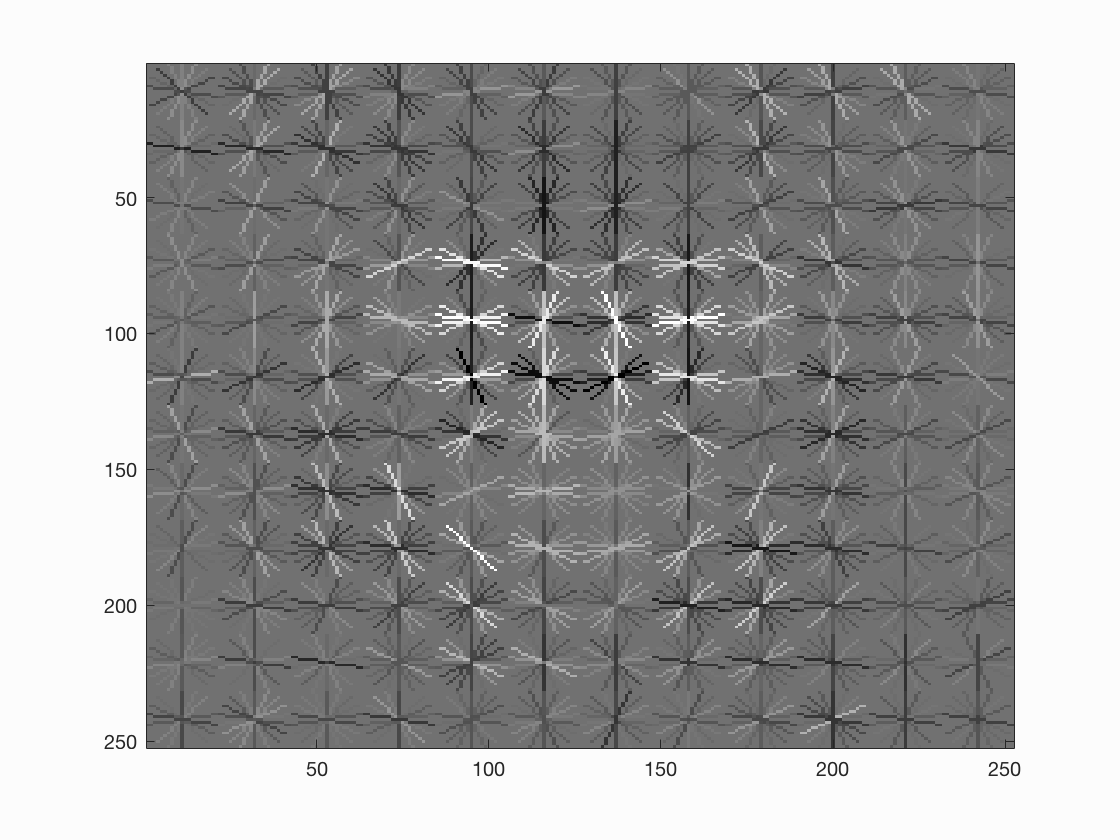
Face template HoG visualization when threshold = 0.7, step size = 6, scale factor = 0.9. We can see that the accuracy improved significantly from single scale.

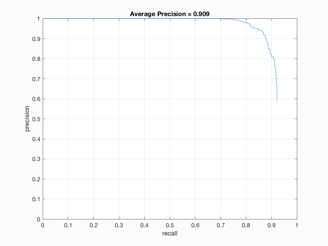
Precision Recall curve for the starter code.

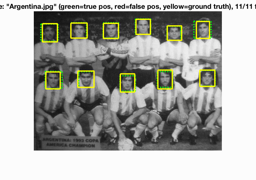
Example of detection on the test set from the starter code.

Face template HoG visualization when threshold = 0.7, step size = 4, scale factor = 0.9. We can see that the HoG visualization gains more details, and there are eyes and mouth.

Precision Recall curve for the starter code.

Example of detection on the test set from the starter code.

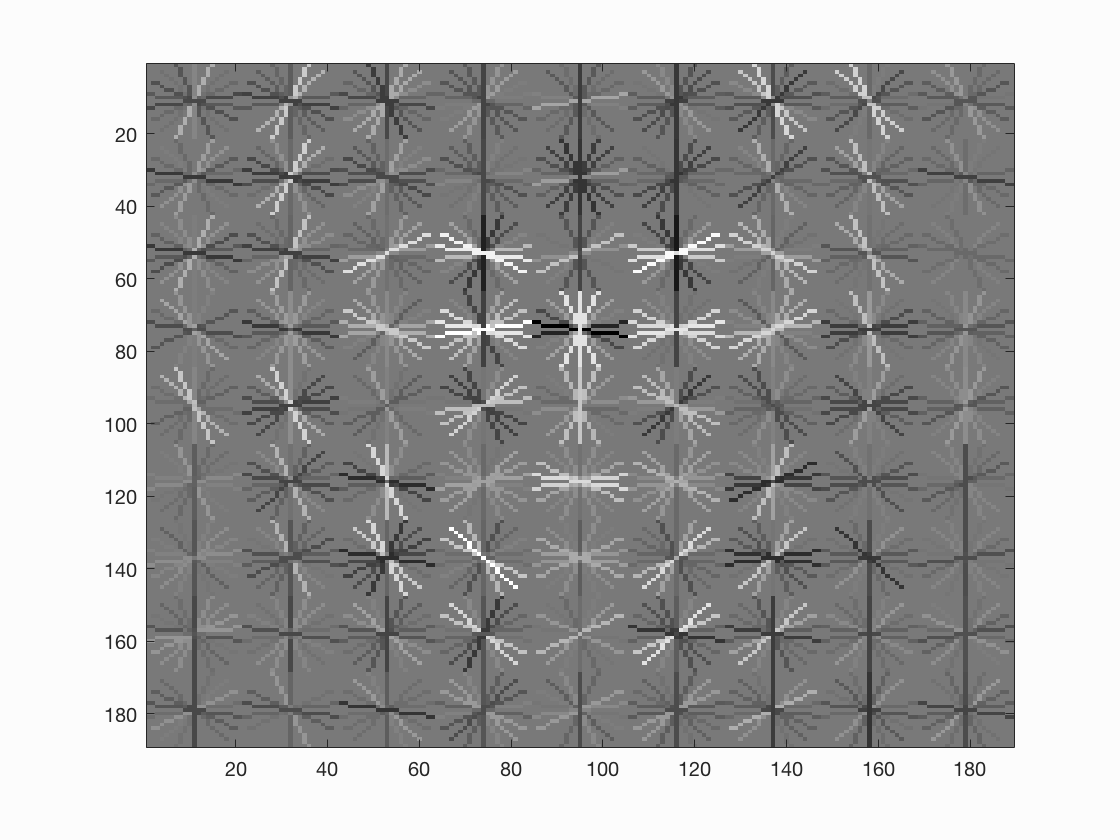
Face template HoG visualization when threshold = 0.7, step size = 3, scale factor = 0.9. We can see that the HoG visualization gains more details.

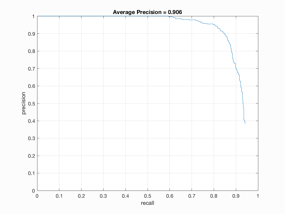
Precision Recall curve for the starter code.

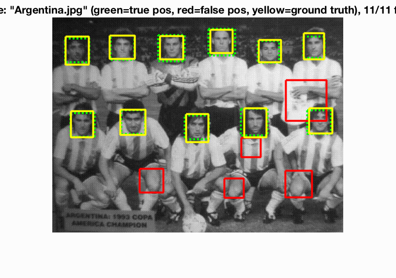
Example of detection on the test set from the starter code. We can see that the performance in this image was much better than before.

Class image. We can see that the faces in the first image were successfully detected, whereas most faces in the second image were not detected.

Extra credit: decision tree

Before I was using linear-svm to train the classifier, but I have also tried using decision tree. Decision tree is a very strong classification algorithm and is very easy to understand, and has been applied in a lot of classification problems.

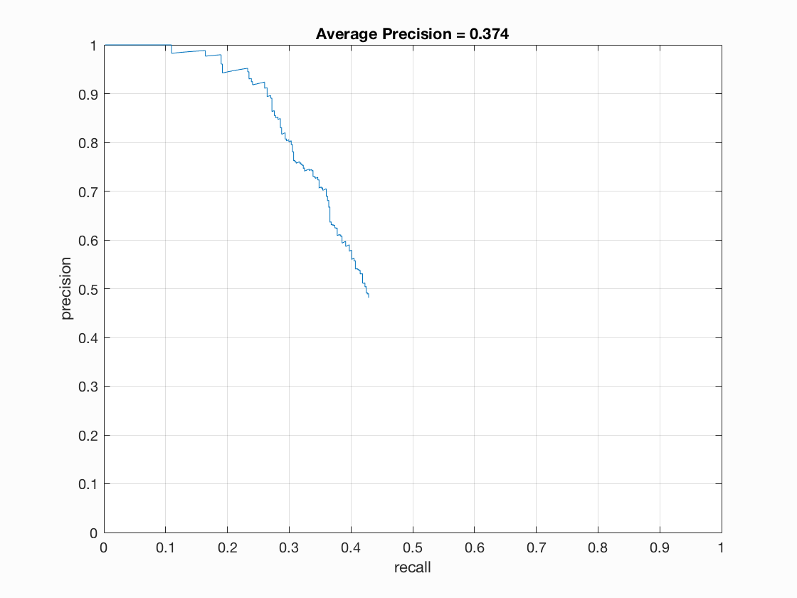
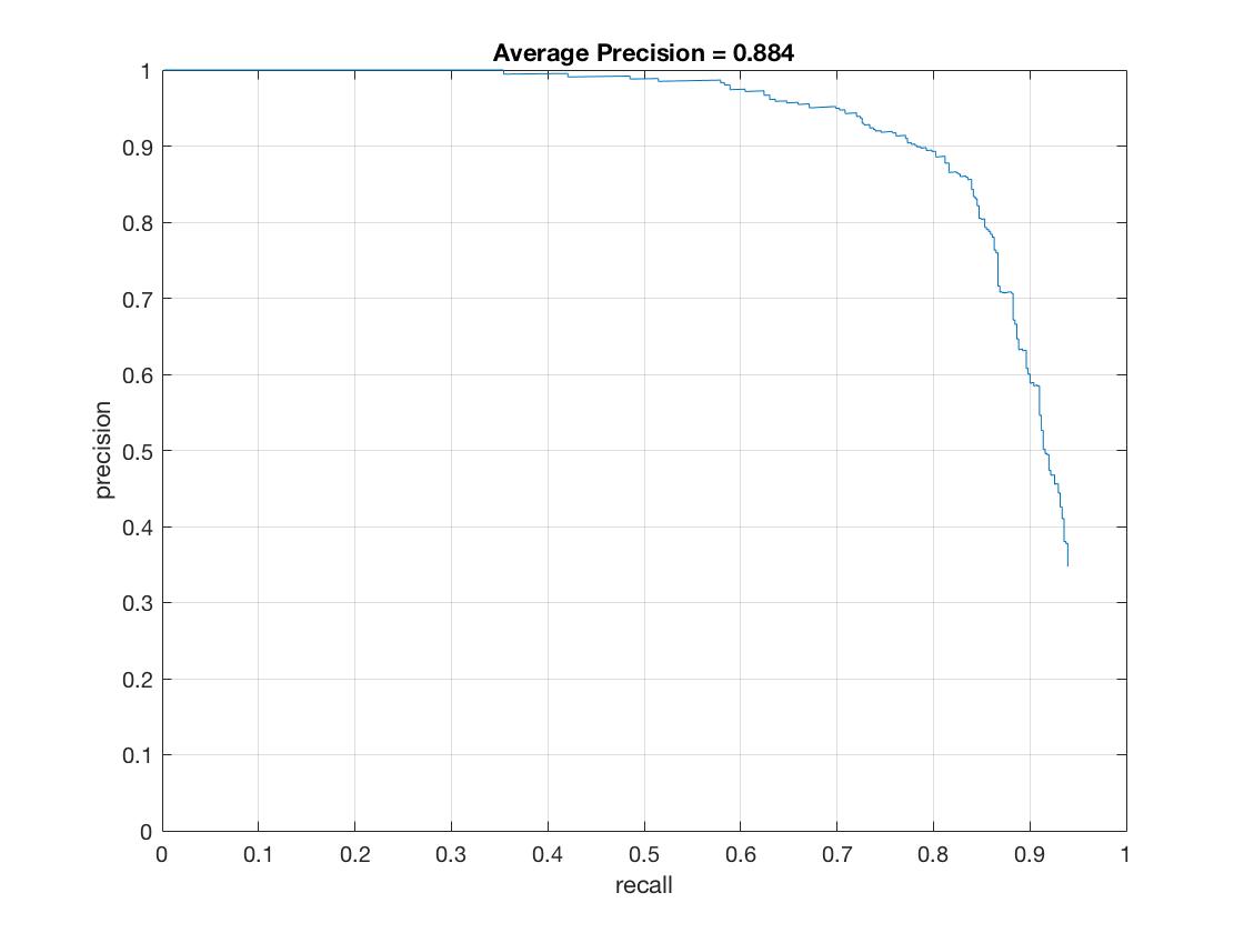
However, the accuracy achieved by decision tree classifier was very low, and I attribute the errors to overfitting. I tried different decision tree, including the default one and a pruned one. I used matlab's cvLoss(tree,'SubTrees','All') function to get the optimal prune level, and the precision / recall curve became slightly better balanced after pruning the decision tree. Even though the overall accuracy was still very low, the curve became flatter and converged in a higher precision. The left chart is the curve for unpruned tree, and the right chart is for pruned tree.

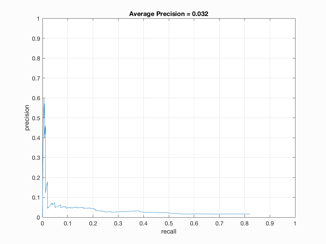
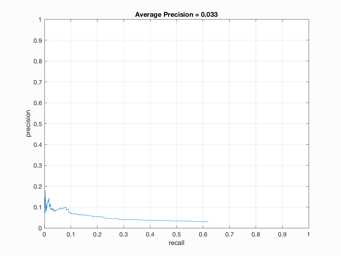
When analyzing the mean square error of the decision trees, I found that the error was very low (0.0038 for unpruned tree and 0.015 for pruned tree), therefore I think the tree might overfitted and the performance should improve significantly with more training samples. Therefore I changed the number of negative sample from 10000 to 20000, and achieved a slightly better accuracy and a better precision-recall curve.

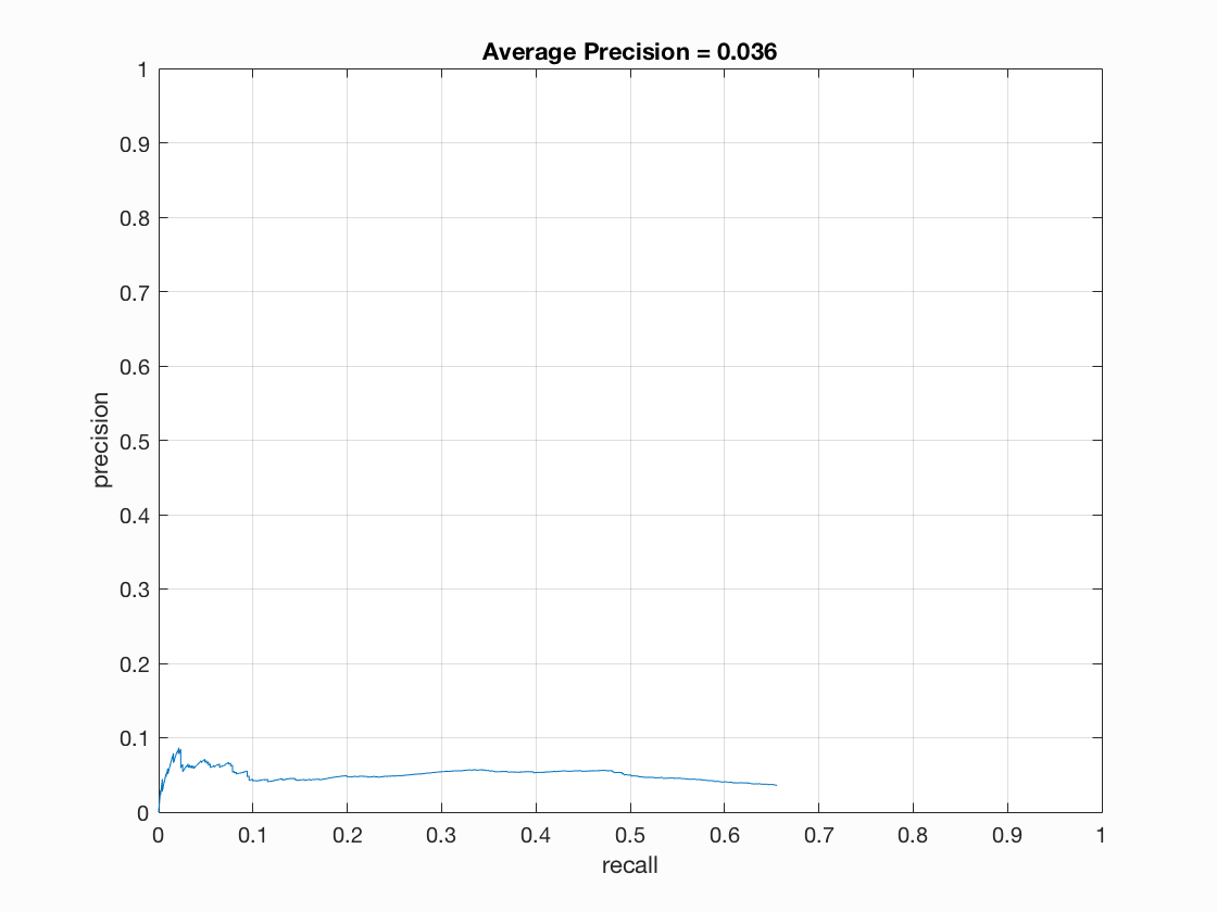
However, overall the decision tree classfier's performance was very low, and it was due to the extremely high false positive rate. I think my current implementation is only slightly better than random, and it might be due to some unknown error within my implementation, or it just need more negative samples to train on.