Project 5 / Face Detection with a Sliding Window
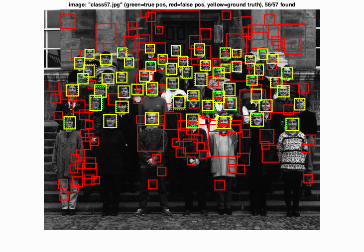
Fig.1. Example of face detection.
The aim of this project is to implement the simple sliding window model in order to realize face detection which means classifying all image patches as being face or not face independently. The pipeline includes handling heterogeneous training and testing data, training a linear classifier and utilizing this classifier to classify millions of sliding windows at multiple scales.
The entire contents of this report are shown as follows:
- Get Positive Features
- Get Random Negative Features
- Linear Classifier Training
- Run Detector
- Results
- Extra Credit - Tuning Various Parameters
- Extra Credit - Sampling Random Negative Examples at Multiple Scales
- Extra Credit - Hard Negative Mining
- Extra Credit - Alternative Positive Training Data
1.Get Positive Features
In this part, the goal is to get all positive training examples which are faces here from 36*36 images. The first step is to open these images and then each face is supposed to be converted into a HoG template using the function vl_hog. Part of the code is shown below.
    ...
    for i=1:num_images
        image=imread(fullfile(train_path_pos,image_files(i).name));
        ...
        HOG_Features_Res=reshape(vl_hog(image,CELLSIZE),1,[]);
        features_pos{i,1}=HOG_Features_Res;
    end
    ...
2.Get Random Negative Features
By contrast, the purpose for this portion is to obtain negative training examples which are non-faces from the images in 'non_face_scn_path'. The images are first converted to grayscale due to the positive training data being merely available in grayscale. Then random negative examples from scenes are sampled and converted to HoG features using vl_hog. The corresponding code is displayed here.
    for i=1:num_images
        image=rgb2gray(imread(fullfile(non_face_scn_path,image_files(i).name)));
        ...
        for j=1:Incre:hy
            for k=1:Incre:wx
                HOG_Features_Res=reshape(vl_hog(image(j:jm,k:km),CELLSIZE),1,[]);
                k_lp=((k-1)/Incre+1);
                j_lp=((j-1)/Incre)*floor((wx-1)/Incre+1);
                features_neg1(j_lp+k_lp,:)=HOG_Features_Res;
            end
        end
        num_per_image=ceil(0.6*size(features_neg1,1));
        features_neg2=features_neg1(datasample(1:size(features_neg1,1),num_per_image,'replace',false),:);
        features_neg=[features_neg;features_neg2];
    end
    features_neg=features_neg(datasample(1:size(features_neg,1),num_samples,'replace',false),:);
3.Linear Classifier Training
For this part, training a linear SVM classifier from the positive and negative examples will be the focus. In the initial step, different labels are assigned to positive and negative HoG features respectively and afterwards utilizing the function vl_svmtrain to train data. The relative code is shown as follows.
    lambda=0.0001;
    data=[features_pos;features_neg];
    data=data';
    label_pos=ones(size(features_pos,1),1);
    label_neg=(-1)*ones(size(features_neg,1),1);
    label=[label_pos;label_neg];
    [w,b]=vl_svmtrain(data,label,lambda);
4.Run Detector
The purpose of this part is to run the classifier on the test set. For each test image, run the classifier at multiple scales and for each scale, get the HoG features, utilize sliding windows to acquire HoG feature patch, and set the threshold to only save the boxes, confidences and image ids above this threshold. Finally, use non_max_supr_bbox to remove duplicate detections. See below for the corresponding code.
    scalebasic=0.95;
    scale_num=41;
    scale=zeros(1,scale_num);
    for i=0:1:(scale_num-1)
        scale(i+1)=scalebasic^i;
    end
    ...
    for i = 1:length(test_scenes)
    ...
        for k=1:1:length(scale)
            HoG_Features=vl_hog(imresize(img,scale(k)),CELLSIZE);
            ...
            for m=1:1:mm
                Ymin=ceil((1+CELLSIZE*(m-1))/(scale(k)));
                Ymax=ceil(CELLSIZE*(m+CellNum-1)/(scale(k)));
                for n=1:1:nm
                    Feat=reshape(HoG_Features(m:m+CellNum-1,n:n+CellNum-1,:),1,[]);
                    tcf=dot(Feat,w)+b;
                    if tcf>threshold
                        Xmin=ceil((1+CELLSIZE*(n-1))/(scale(k)));
                        Xmax=ceil(CELLSIZE*(n+CellNum-1)/(scale(k)));
                        cur_bboxes=[cur_bboxes;Xmin,Ymin,Xmax,Ymax];
                        cur_confidences=[cur_confidences;tcf];
                        cur_image_ids=[cur_image_ids;{test_scenes(i).name}];
                    end
                end
            end
        end
        ...
        [is_maximum] = non_max_supr_bbox(cur_bboxes, cur_confidences, size(img));
        ...
    end
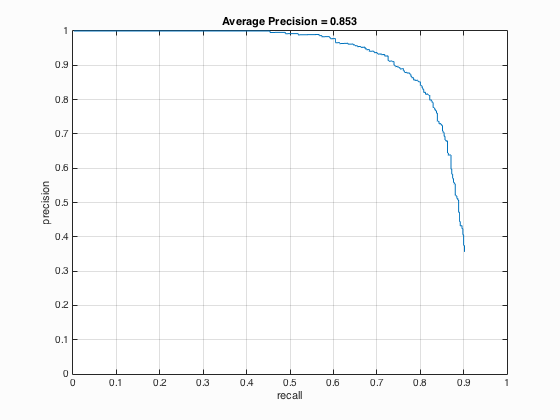
5.Results
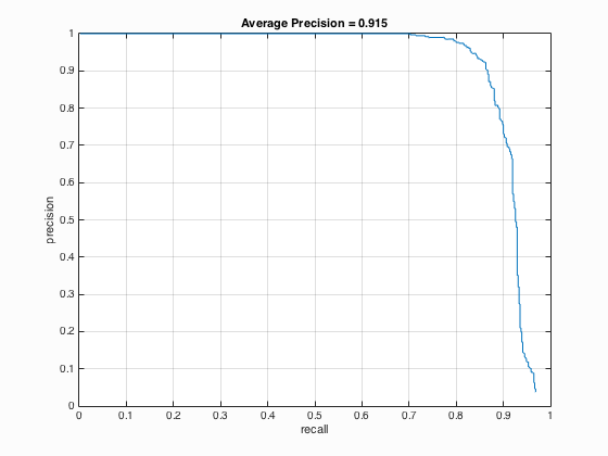
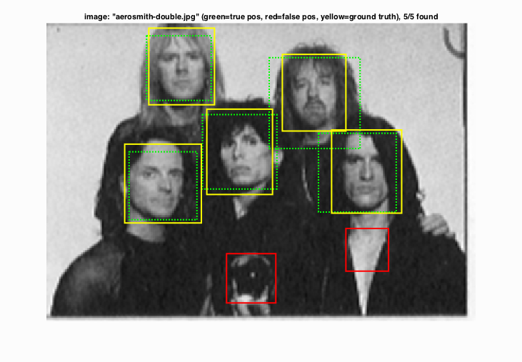
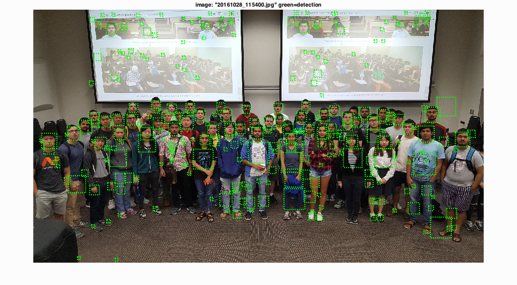
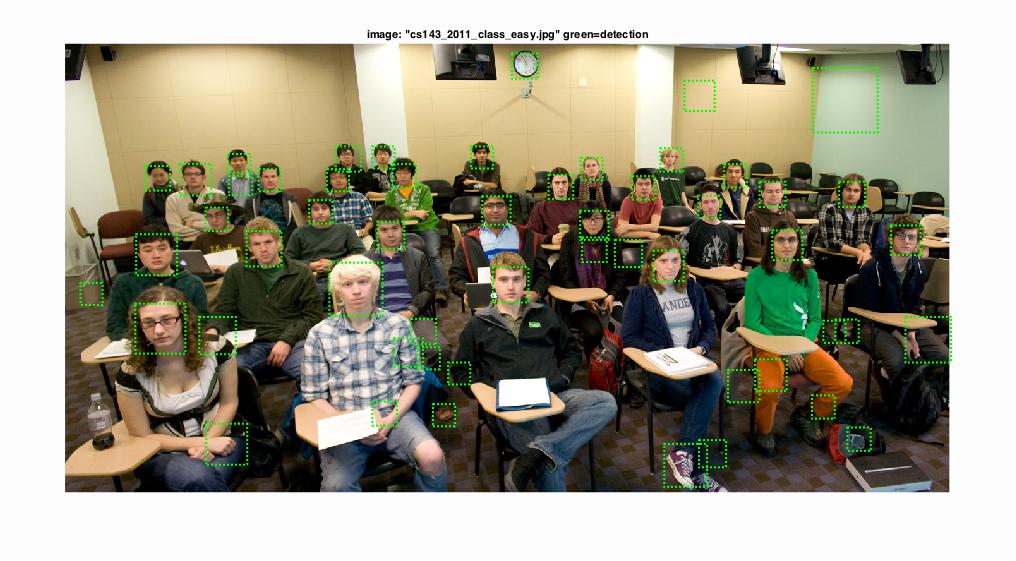
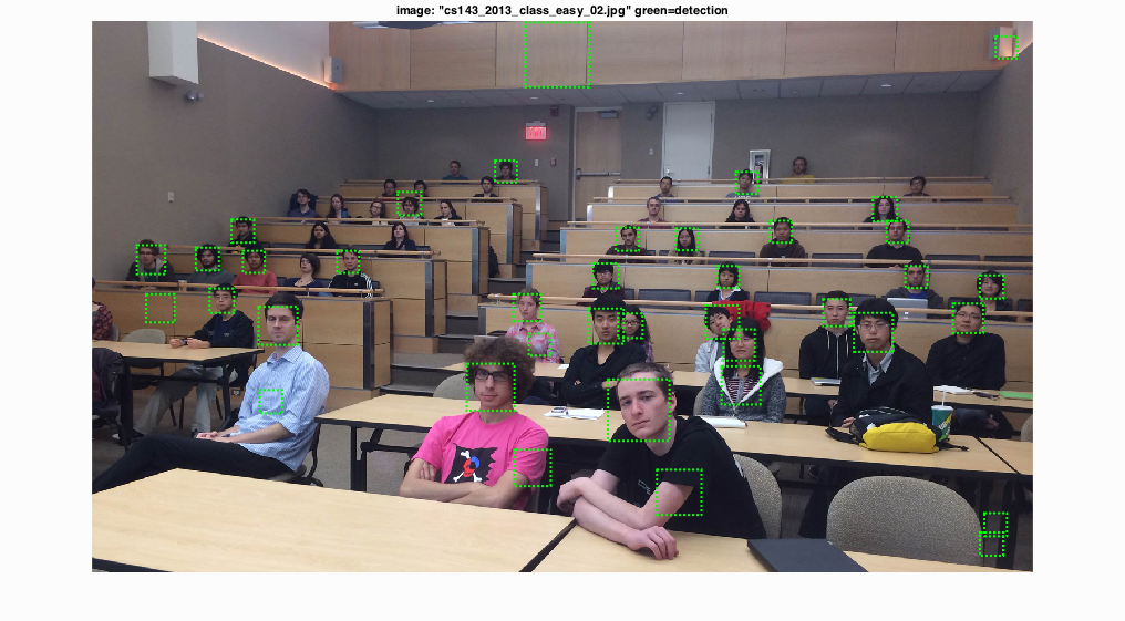
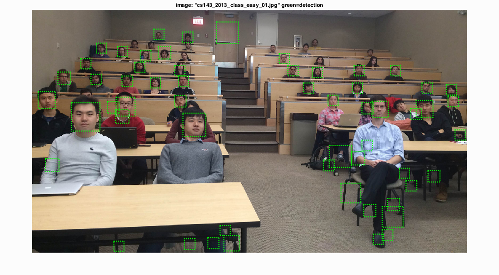
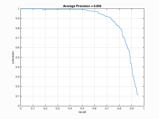
The following results of CMU+MIT test scenes using parameters set as follows: HoG cell size equals to 3, the number of negative examples is 30000, lambda is 0.0001, the number of scales utilized in run detector is 41 times and the threshold is 0.2. The average precision is approximately 91.5 % for CMU+MIT test scenes. The parameters for extra test scenes: HoG cell size equals to 6, the number of negative examples is 10000, lambda is 0.0001, the number of scales utilized in run detector is 41 times and the threshold is 0.8. The results are quite good for both CMU+MIT and extra test scenes. It can be seen that nearly all of the faces have been detected for both image sets.
|
|
Fig.2. The results of CMU+MIT test scenes.
|
|
Fig.3. The results of extra test scenes.
6.Extra Credit - Tuning Various Parameters
6.1. num_negative_examples
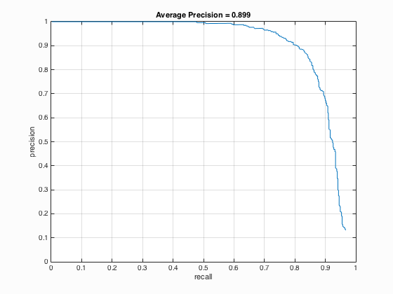
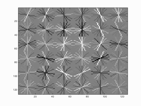
Table 1. The relationship between the number of negative examples and the average precision.
| num_negative_examples | Average Precision | HoG_Template |
| 10000 |

|

|
| 20000 |

|
|
| 30000 |
|
|
From the Table 1 above, it can be seen that with the increase of the number of negative examples from 10000 to 30000, the average precision has also enhanced by approximately 1.1 % which is not that obvious.
6.2. Multiscales in run_detector.m
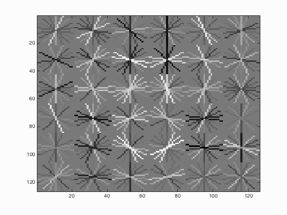
Table 2. The relationship between the number of different scales used and the average precision.
| Number of Scales | Average Precision | HoG_Template |
| 81 |
|
|
| 61 |
|
|
| 41 |

|

|
| 21 |
|
|
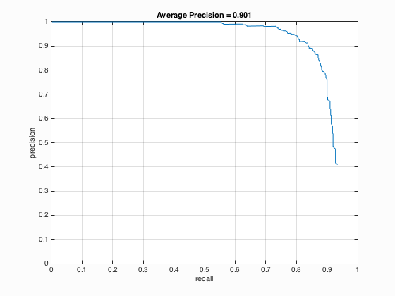
It is undoubted that the use of multiscale with small step size is able to increase the average precision. It is indicated from table 2 that when the number of different scales is set to 81, the average precision is 90.1 % which corresponding to the statement that with small step size the paper's performance could be matched with average precision above 90 %. Besides, when the number of different scales is enhanced from 21 to 41, there is a relatively evident increment in average precision which is around 4 % while above 41, the augment is not clear.
6.3. Threshold in run_detector.m
Table 3. The relationship between the threshold used and the average precision.
| Threshold | Average Precision | HoG_Template |
| 0.8 |

|
|
| 0.5 |

|
|
| 0.2 |
|
|
| 0 |

|
|
It is able to be concluded that if the threshold is lowered, the number of detections increases which will surely lead to the increment of average precision but at the same time, more false positives will be returned.
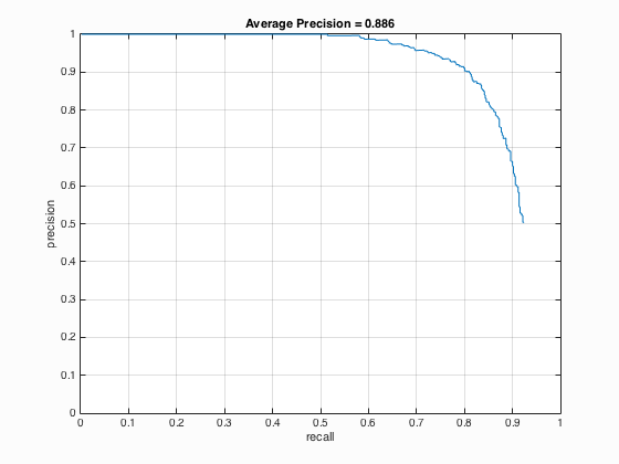
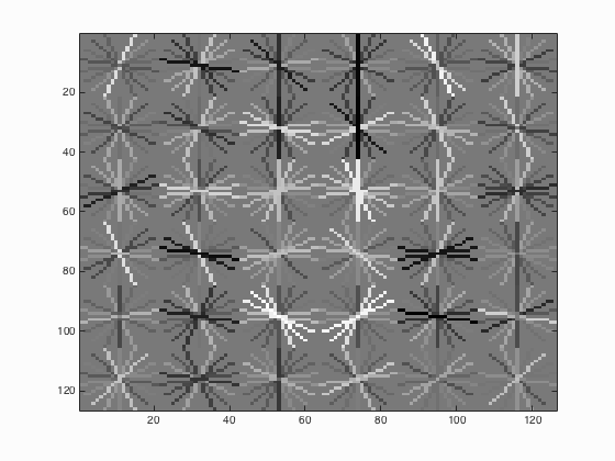
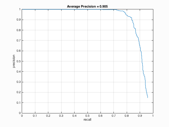
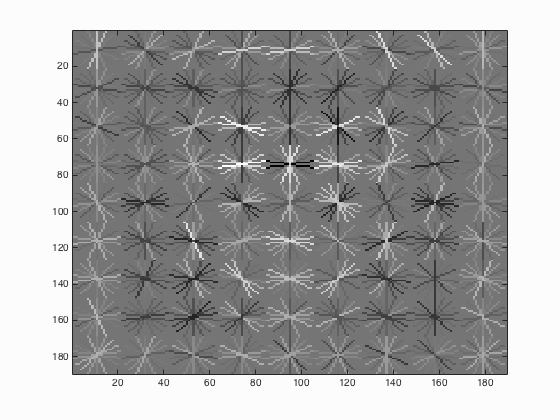
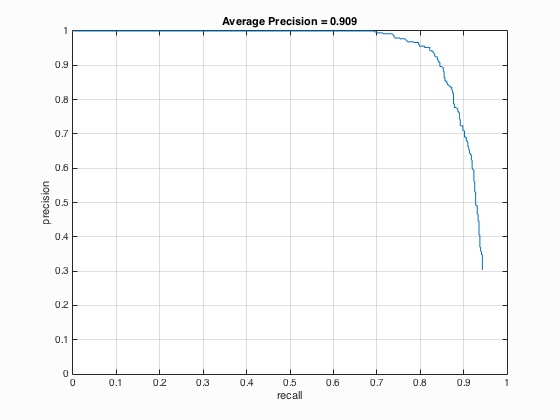
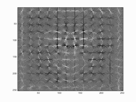
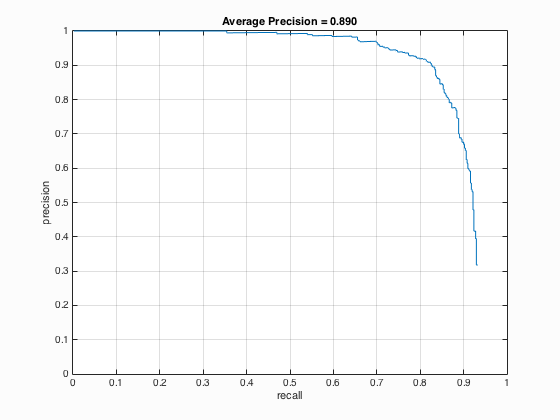
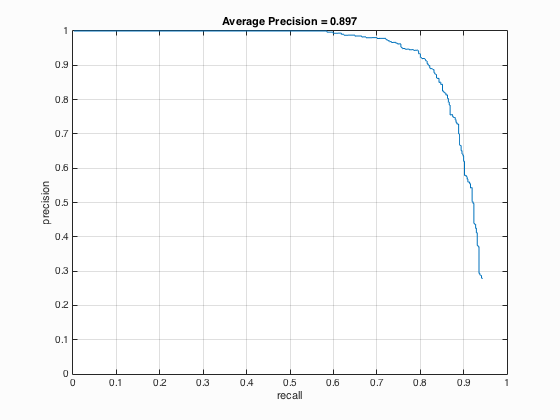
6.4. hog_cell_size
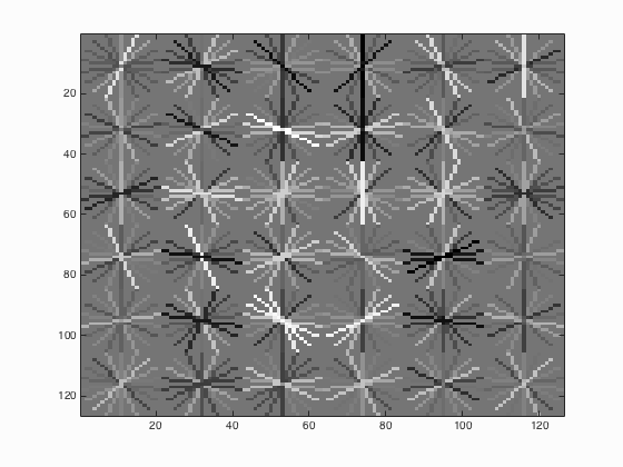
Table 4. The relationship between the cell size and the average precision.
| HoG Cell Size | Average Precision | HoG_Template |
| 6 |
|
|
| 4 |
|
|
| 3 |
|
|
It can be seen from the above Table 4 that the average precision is inversely proportional to the cell size which means with the decrease of cell size from 6 to 3, the average precision increases from 88.6 % to 90.9 %.
7.Extra Credit - Sampling Random Negative Examples at Multiple Scales
Table 5. The relationship between the number of scales when sampling random negative examples and the average precision.
| Number of Scales | Average Precision | HoG_Template |
| 1 |
|

|
| 5 |
|
|
The results from Table 5 above indicate that sampling random negative examples at multiple scales shows better performance which means higher average precision than the single scale but the variation is not that evident.
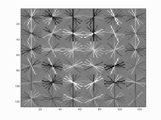
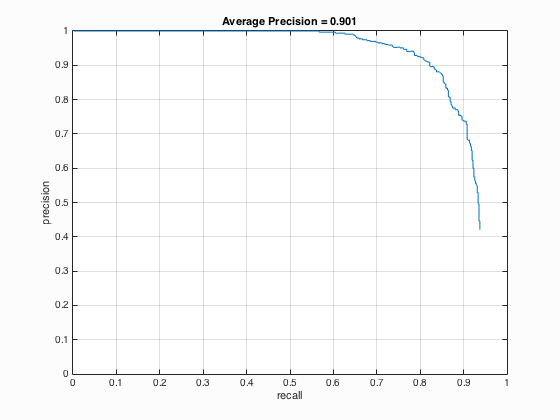
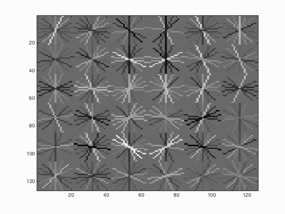
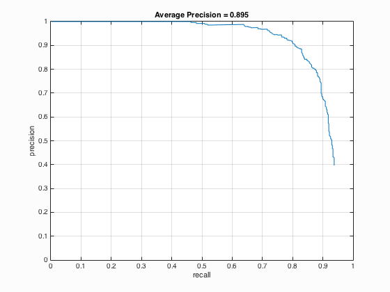
8.Extra Credit - Hard Negative Mining
In this section, negative images are used to test the SVM and then those hard negatives are added to the original negative features in order to the increment of negatives. The relative code as well as results are shown as follows.
    for i=1:1:size(features_neg,1)
        tcf=dot(features_neg(i,:),w)+b;
        if tcf>threshold
            features_neg_new=[features_neg_new;features_neg(i,:)];
        end
    end
    ...
    [w,b]=vl_svmtrain(train_example,train_label,lambda);


|

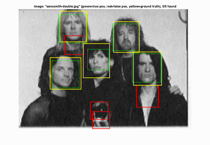 |
Fig.4. Results before (upper) and after (lower) using hard negative mining for CMU+MIT test scenes.

|
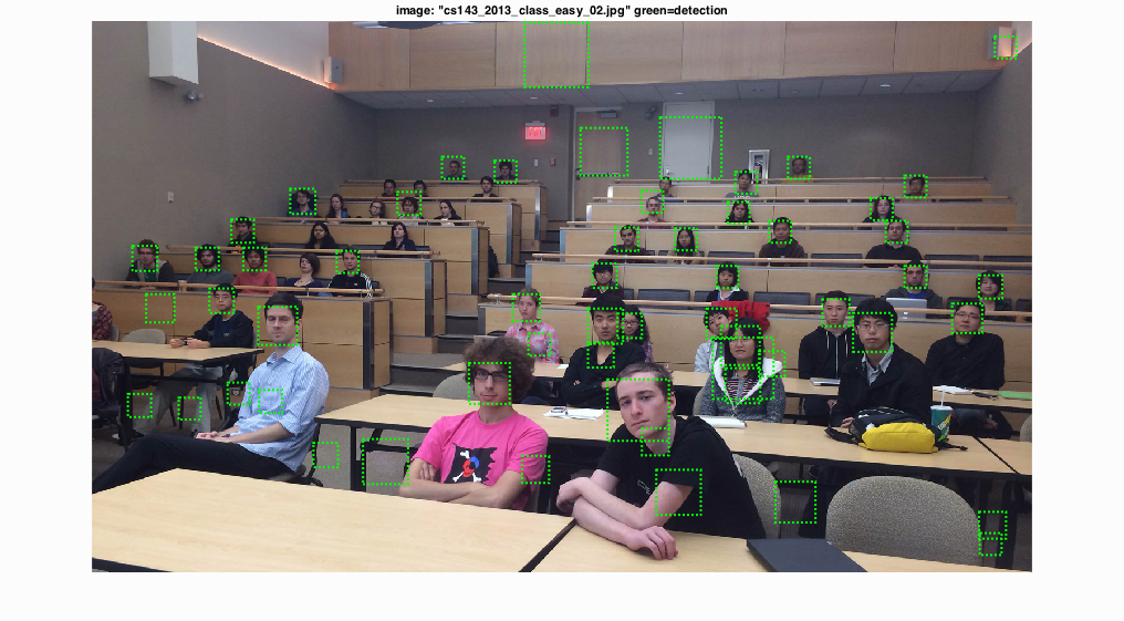 |
Fig.5. Results before (upper) and after (lower) using hard negative mining for extra test scenes.
From the outcomes above, it can be seen that after using hard negative mining, the performance seems better. For CMU+MIT test scenes, the accuracy increases from 88.9 % to 90.3 % and for extra test scenes, there are more correct detections.
9.Extra Credit - Alternative Positive Training Data
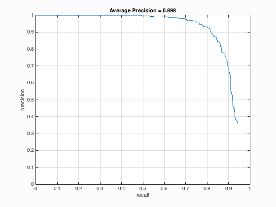
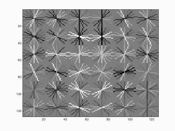
I implemented both the Yale Face Database B and ATT "The Database of Faces". For Yale Face Database B, it contains 16128 images of 28 human subjects under 9 poses and 64 illumination conditions. The results show that the average precision decreases from 88.6 % to 85.6 %. For ATT "The Database of Faces", it includes ten different images of each of 40 distinct subjects and some of them varies the lighting, facial expressions and details. As shown in 9.2, the average precision enhances from 88.6 % to 89.8 %. The relative code is shown below:
    image_files = dir( fullfile( train_path_pos, '*.jpg') ); %Caltech Faces stored as .jpg
    ...
    for i=1:num_images
        image=imread(fullfile(train_path_pos,image_files(i).name));
        image=single(image)/255;
        HOG_Features_Res=reshape(vl_hog(image,CELLSIZE),1,[]);
        features_pos{i,1}=HOG_Features_Res;
    end
    ...
    for i=1:39
        path_pos_yale=fullfile(train_path_pos_yale,strcat('yaleB',int2str(i)));
        image_files_yale=dir(fullfile(path_pos_yale,'*.pgm'));
        for j=1:length(image_files_yale)
            img=imread(fullfile(path_pos_yale,image_files_yale(j).name));
            img=single(imresize(img,[TempSize,TempSize]))/255;
            HOG_Features_Res_Yale=reshape(vl_hog(img,CELLSIZE),1,[]);
            features_pos=[features_pos;HOG_Features_Res_Yale];
        end
    end
9.1. Yale Face Database B


|
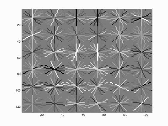 |
Fig.6. Results before (upper) and after (lower) using Yale Face Database B for CMU+MIT scenes.
9.2. ATT "The Database of Faces"
|
Fig.7. Results after using ATT "The Database of Faces" for CMU+MIT scenes.