Project 5 / Face Detection with a Sliding Window
Contents
1. Get Training Features and Classify Training
The first is to extract HoG features from the face images and non-face images and thus to form training features. For face images, they are of the same size. So we can just loop through
each image and call vl_hog function to extract the hog feature. For non-face images, they are of different dimensions. And the number of non-face images are much less than that
needed to get enough negative training features. The strategy is to crop different patches with 36x36 size from each non-face images, and extract hog feature from each patch as a negative
training features. In this part, the fundamental parameter is the size of each hog cell (tested with 6, 4, 3) and the number of negative features (usually 2e+4 or 1e+4).
SVM is initially used for classification. The parameter lambda is important. Too large values have bad training results. Too small would introduce overfitting modestly in my implementation.
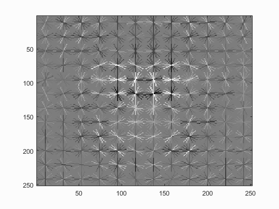
The range can be first tuned by looking at the evaluation on the training error. Small errors would generate a good separability on the positive and negative features, shown in Fig. 1. Then try different values in the right range on the testing images. And based on the experimental results,
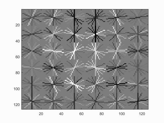
it can be set to 1e-4 to 1e-6, resulting good classifications. With the following paramters, the learned detector can be visulized in Fig. 2.
feature_params = struct('template_size', 36, 'hog_cell_size', 3);
lambda = 1e-5;
num_negative_examples = 20000;

2. Testing and Results
After training, we get the weights and bais, using which we can classify a new feature example. For each testing image, we run the sliding window detection on multiscales. For each scale, the global hog feature is first extracted. And then a sliding window goes through the global hog features in top-down, left-right manner. The window size is the same as the face images. Thus each window generates a feature example, which is then put to the SVM classifier to find whether it is a face nor not. And threshold parameter is set to cut off low score feature examples. For positive classification windows, the locations are recorded. After detecting one image, non_max_supr_bbox is used to remove duplicate detections.
For the threshold, it is used to remove low confidence detections. In general, any positive value works. In my implementation, the good values are in the range of [0.1,0.5]. The choice of
multiple scales matters. Densely selected scales tend to generate better results but require high computation. Due to hardware limitation, I let each image only go 4 different scale detection.
I tried the following scales, among which scaleV = [1,0.7,0.5,0.3] provides highest precision.
scaleV = [1,0.8,0.6,0.4];
scaleV = [1.1,0.9,0.7,0.5];
scaleV = [1,0.7,0.5,0.3];
With the above implementation, I ran detection for different parameter sets. The main parameters are the size of hog size, lambda, number of negative training samples, scales and threshold.
I have talked about the choice of scales and threshold. For the number of negative training samples, large number would increase testing precision. However, as the non-face images are limited,
generating hundreds of thousands of negative samples would not help either. In my implementation, num_negative_examples = 20000 provides good precisions.
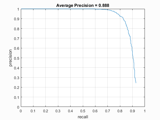
To find out how lambda affects the classification result, I used the following parameters and ran the classification with lambda from 1e-1 to 1e-7. The overall precision for the
testing set is shown in Fig. 3. Generally lower values provide higher precisions.
feature_params = struct('template_size', 36, 'hog_cell_size', 4);
lambda = 1e-4;
num_negative_examples = 20000;
scaleV = [1,0.7,0.5,0.3];
threshold = 0.3;

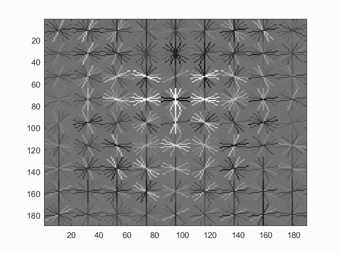
For the hog cell size, I tried 6, 4 and 3. Smaller sizes provide larger dimensional features with fine details to generate higher precisions, which are shown in Fig. 4 by comparing the learned
detector with differnt hog cell sizes. And table 1 shows the precision for different hog size with lambda = 1e-5
| hog cell size | 6 | 4 | 3 |
| Precision | 79.8% | 87.2% | 88.8% |
|
|
|
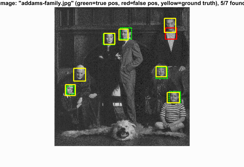
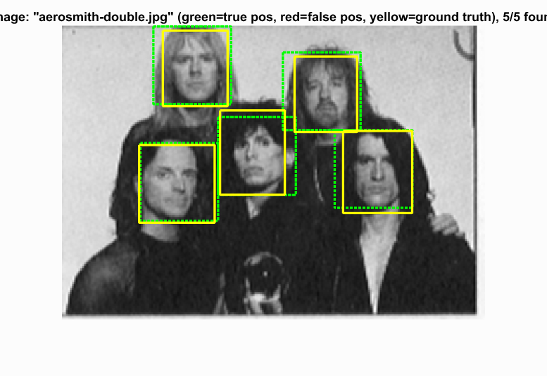
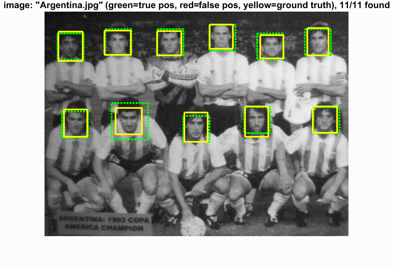
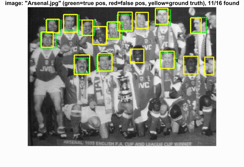
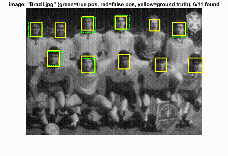
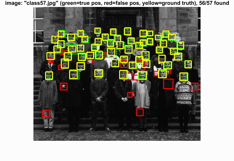
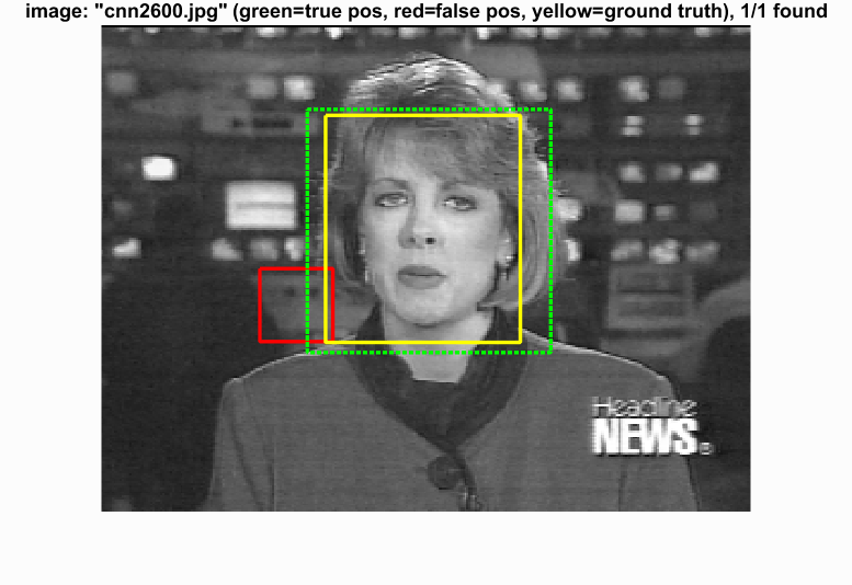
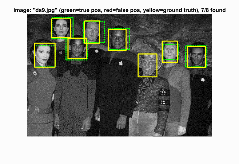
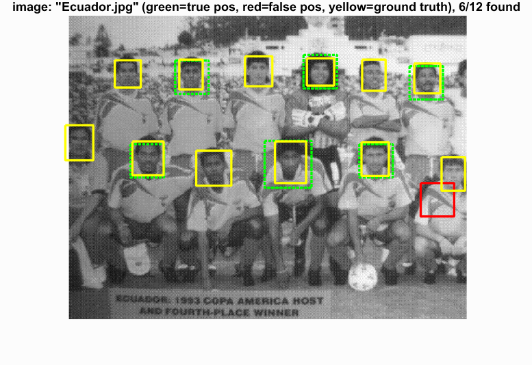
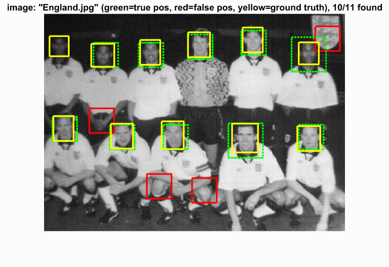
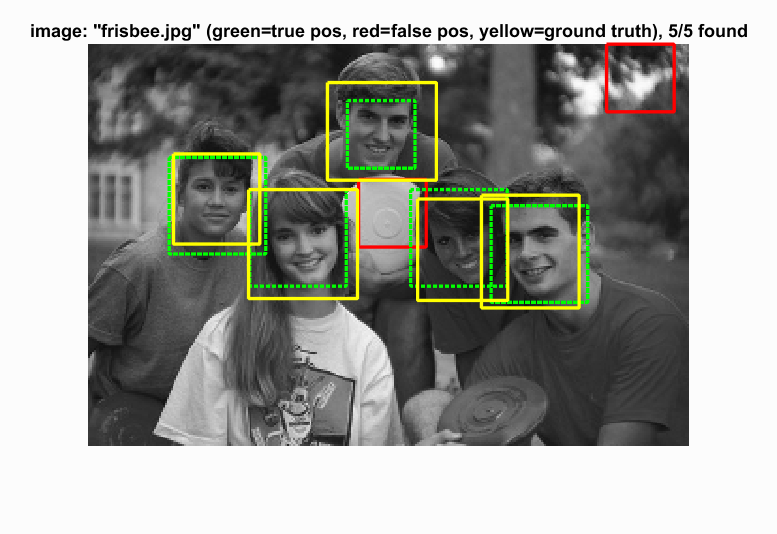
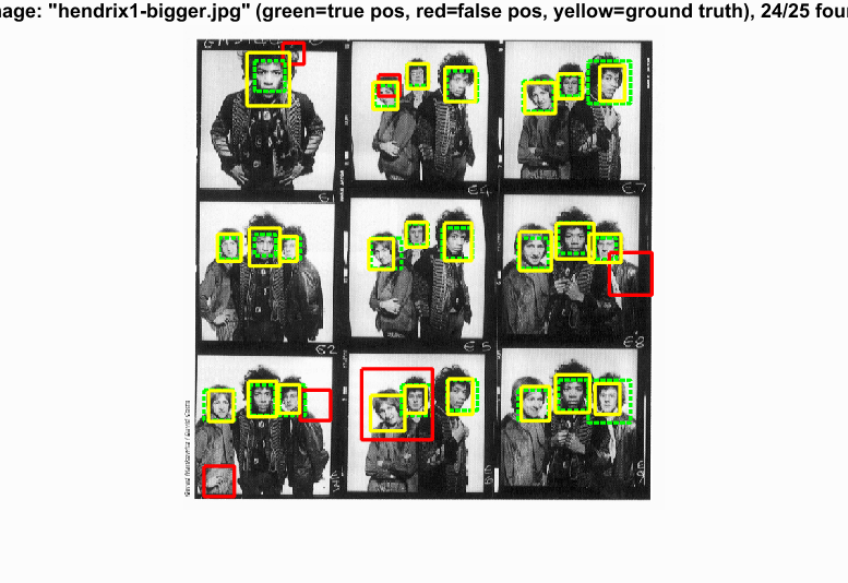
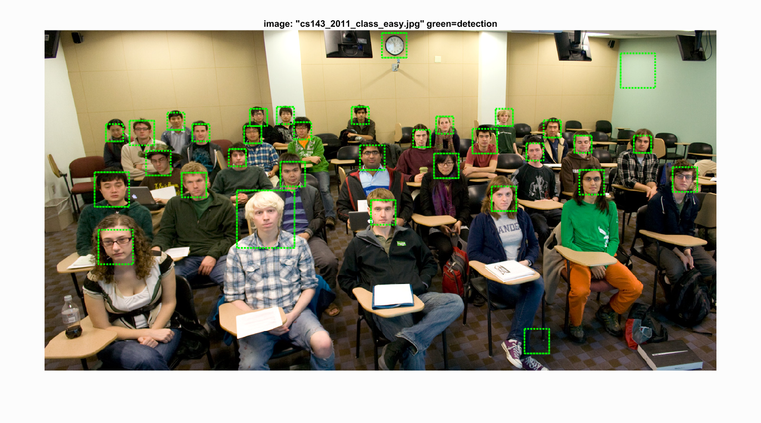
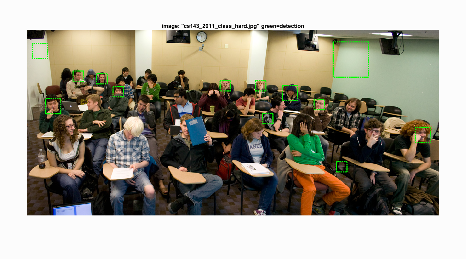
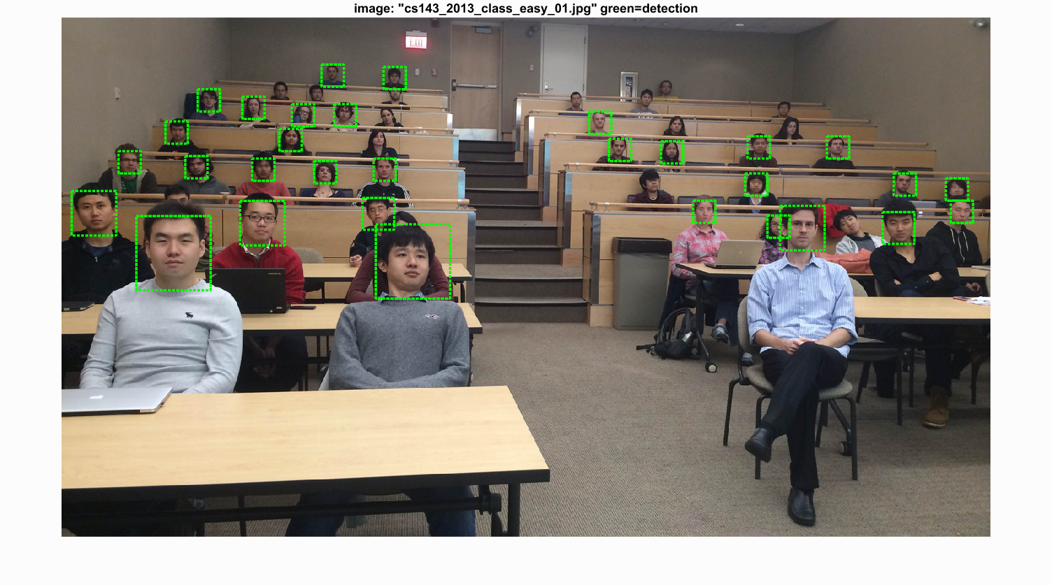
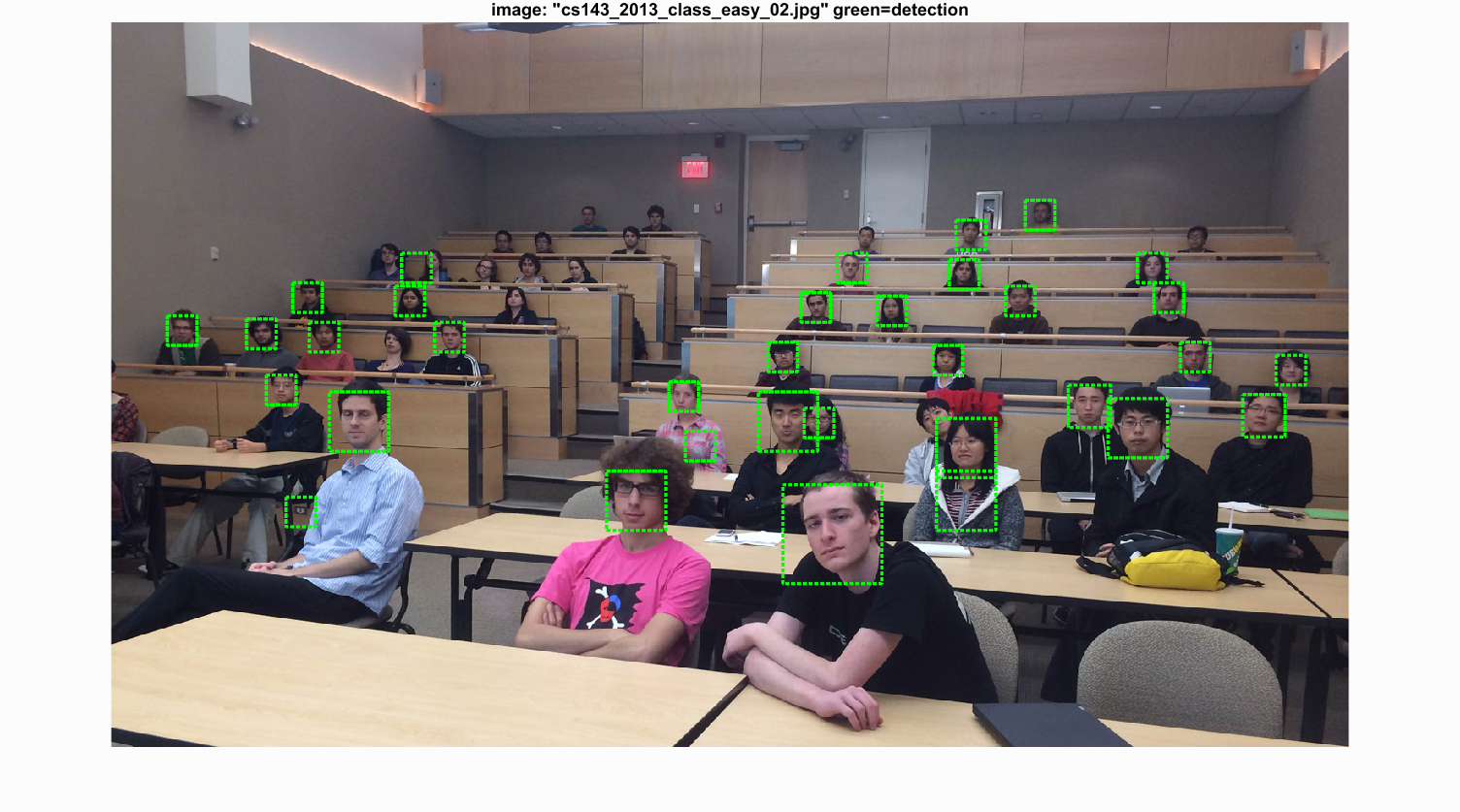
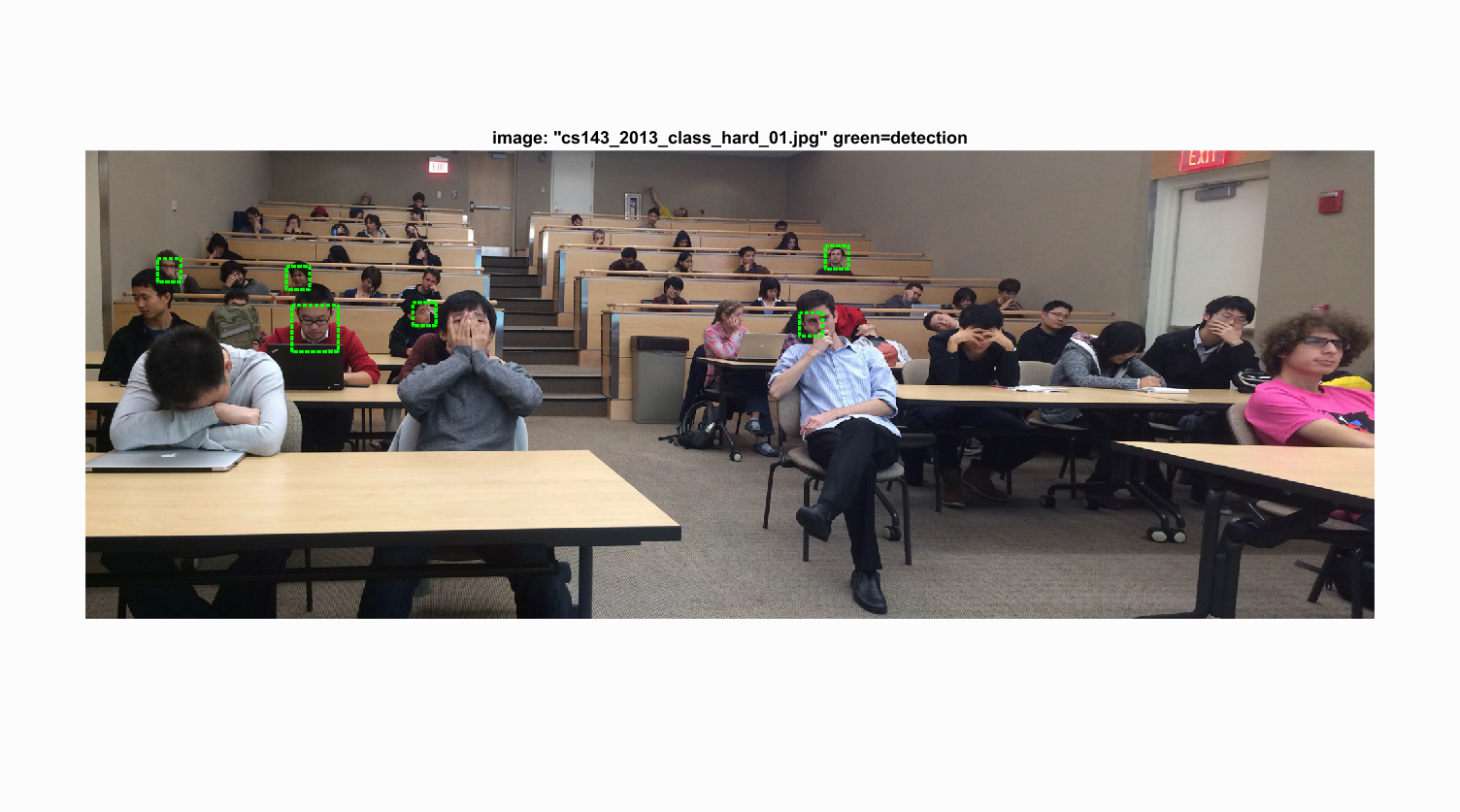
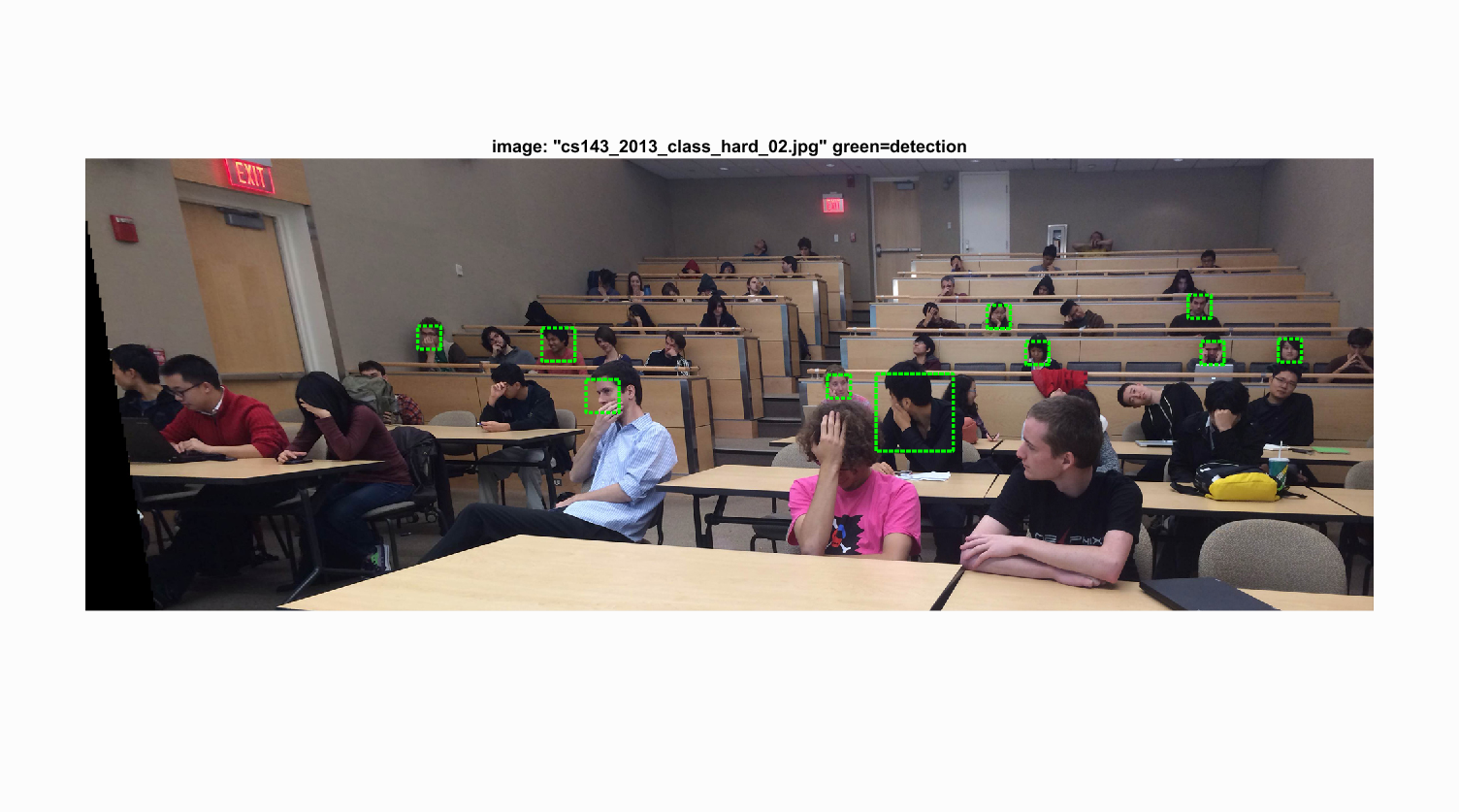
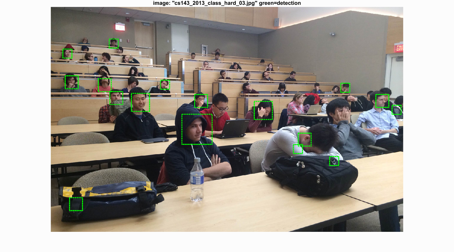
The following results are from the detection with 88.8% precision. For detection with class images, the threshold is set to 1 to make the result cleaner.
Example of detections.
|
|
|
|
|
|
|
|
|
|
|
|
|
|
|
|
|
|
3. Extra credit/Graduate credit
- Implement a HoG descriptor yourself.
HoG.m. For each input image, the gradient at pixel level is calculated by matlab
imgradient function. Then for each dividied cell, the gradients for all the cell pixels are counted into a histogram
of bin size 36, with each bin representing 10 deg segment. Last the histogram is vectorized and normalized. For the whole image,
all the histograms form up the HoG feature.
Using costomized HoG to extract features and detect faces is in
proj5_hog.m. For one run with the following parameters, it reaches to 0.716 precision. As I refine the 'hog_cell_size' to
3, the precision goes up to 0.855 without any parameter tuning. The costomized HoG extractor is as powerfull as the on in VLFEAT library.
feature_params = struct('template_size', 36, 'hog_cell_size', 3)
num_negative_examples = 10000;
lambda = 1e-5;
scaleV = [1,0.7,0.5,0.3];
threshold = 0.1;
- Use additional classification schemes. (incomplete)
run_detector_knn.m. Matlab function knnsearch is used to find closest examples from the training features.
However, it is much slower than SVM classifier. The performance is unknown due to time limit.
- Interesting features and combinations of features.
proj5_more.m. The feature is extracted by calling CostomizedFeature.m.
What it does is to attach normalized intensity from the input image to the vectorized hog feature. The extracted feature from each image needs to be normalized before training SVM, otherwise, the
trained weights and bias are NAN. With this feature for face detection, the precision is similar to that with just hog feature, sometimes even lower, showing that the hog feature already captures the important
features of faces.