Yishan Chen

Get Positive Features

This part of code loads cropped positive trained examples (faces) and converts them to HoG features with a call to vl_hog. The followings are the detailed steps:

1. Tterate through all images.
2. For each image, computes the HOG features for the specified HOG cell size (6 as default) by calling the function vl_hog.
3. The size of the HOG matrix is 6x6x31. Convert this matrix to a 1116 vector.
4. Save the vector into feature matrix and finally get an N by 1116 dimension matrix, where N is the number of faces.

Get Random Negative Features

This part of code samples random negative examples from scenes which contain no faces and converts them to HoG features. The followings are the detailed steps:

1. With the given number of random negatives to be mined, compute the average number of features for each image.
2. Since some images might be too small to find enough features, add an additional number of features for each image.
3. Repeat the process metioned in the chapter "Get Positive Features" and finally get a N by 1116 feature matrix.

Classifier Training

This part of code trains a linear classifier from the positive and negative examples with a call to vl_svmtrain. This function trains a linear Support Vector Machine (SVM) from the data vectors and labels. The followings are the detailed steps:

1. Transpose the positive and negative feature matrix and combine them together.
2. Set the label of positive features to be 1 and negative features to be -1.
3. Set lambda as 0.0001 and call the vl_svmtrain function to get training results.

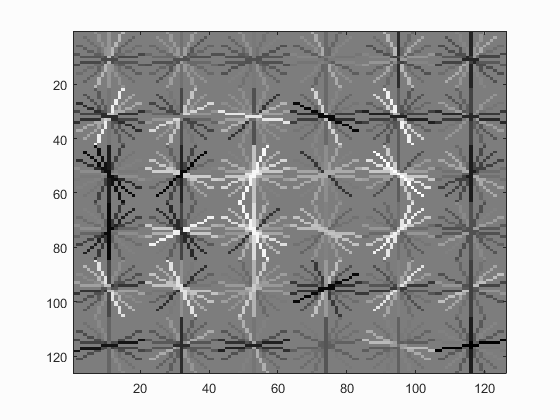
The following is the face template HOG visualization:

Run Detector

This part of code runs the classifier on the test set. For each image, run the classifier at multiple scales and then call non_max_supr_bbox to remove duplicate detections.

Single scale

The first step of this part is to implement the function to detect features at a fixed single scale. The first part of this step is to compute the HOG features of each images. The process of this step is same to the process mentioned in the chapter "Get Positive Features". At the end of this part, a feature matrix with N by 1116 dimension is computed.

Use the W and B calculated by vl_svmtrain to compute the confidence. The confidence equals dot(W, features) plus b. If the confidence is above the setting threshold, then the bounding box of the detected feature is saved. In the end, non-maximal suppression was done to select more confidence bounding boxes.

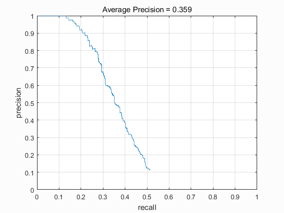
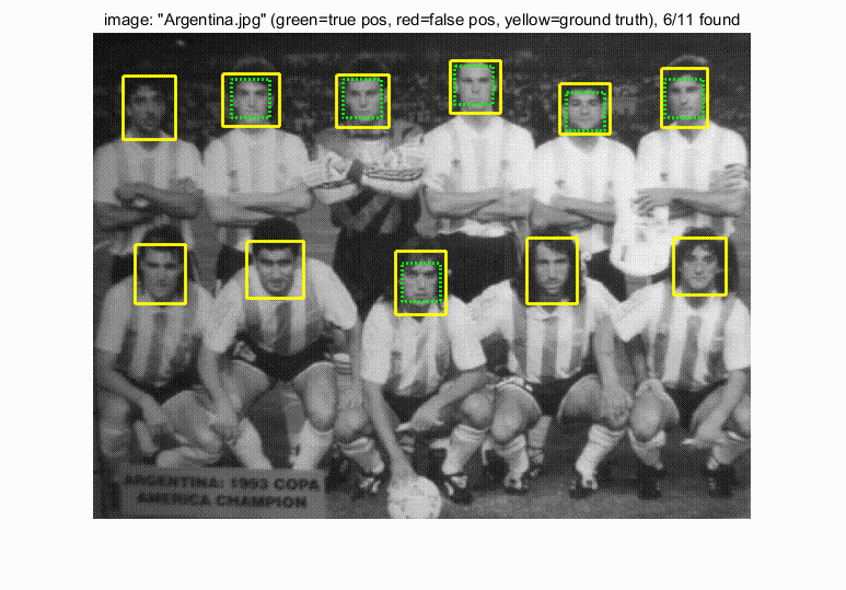
The results for a single scale detector have the average precision of 0.359 when scale is 1:

The following is the detection result for image Argentina:

Multiple scales

The next step is to modifiy the function to multiple scales. Start detecting from a select scale size and process the image as the same step in single scale. When finished, scale the picture with the value of scale step (e.g. 0.8) times original scale size for the next loop. Loop until the image is smaller than the template size (probably 36).

Since the images are scaled, the results of bounding boxes are also scaled. Therefore, the bounding boxes need to be scaled back before saved.

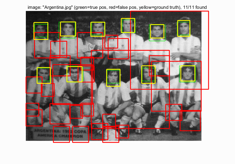
The results for multiple scales detector have the average precision of 0.857 when the step size is 6, the start scale is 1 and the scale step is 0.8:

The following is the detection result for image Argentina:

Extra credit: Hard Negative Mining

Hard negative mining can be implemented to improved classification accuracy. The followings are the steps of hard negative mining:

1. Train all positive and negative examples as before to get a linear Support Vector Machine classifier.
2. Run this classifier on the negative examples to get new negative features.
3. Combine the original and the new negative features together as the modified negative features.
4. Train the positive and the modified negative features together to get a new linear Support Vector Machine classifier.
5. Run the new classifier on the test examples to get results.

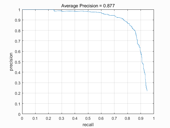
The start scale is 1 and the scale step is 0.8 for both hard mining and testing. The cell size for HOG is 6. When the thresholds of hard mining and testing are both -0.5, the performance of the funcion don't vary much. The accuracy of the results is 0.855, even 0.002 lower than the accuracy without hard mining. Therefore, I change the threshold of hard mining. The function works quite well when the threshold of hard negative mining is 0 and the threshold of testing is -0.5. The average precision is 0.877 after implementing hard mining:

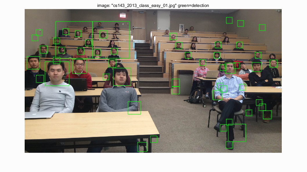
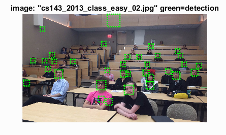
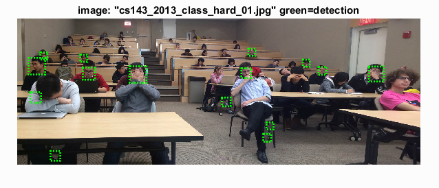
The followings are some detection results:

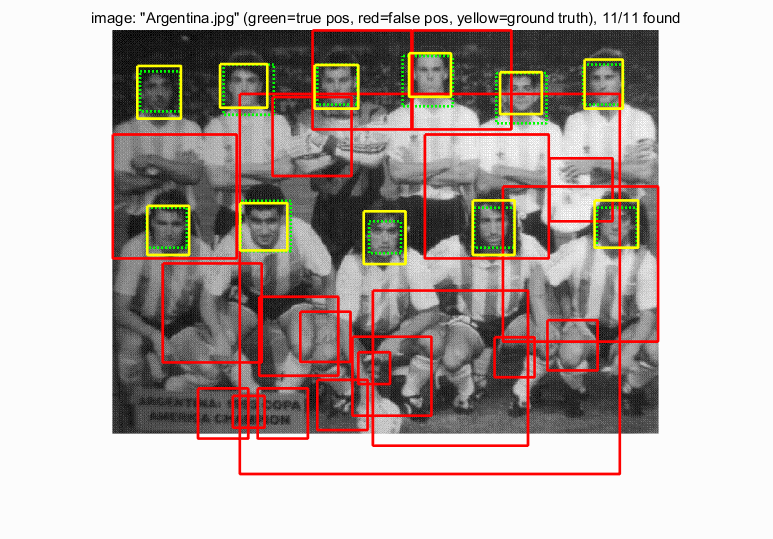
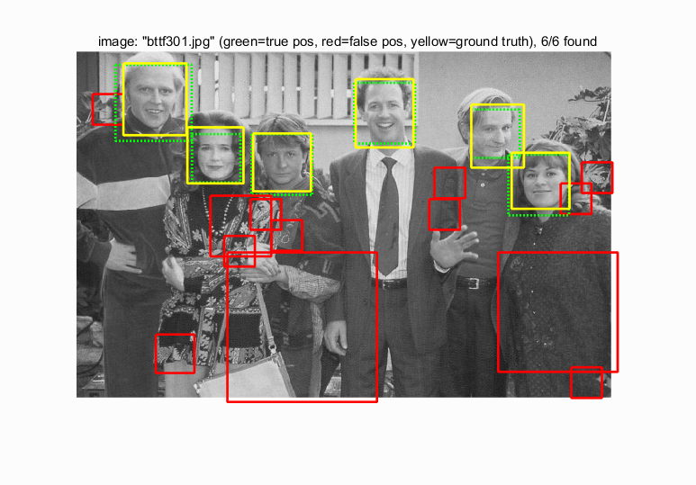
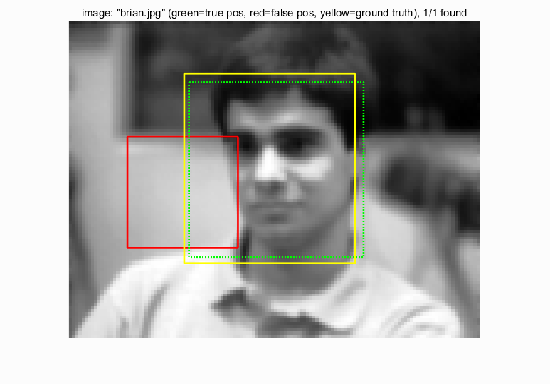
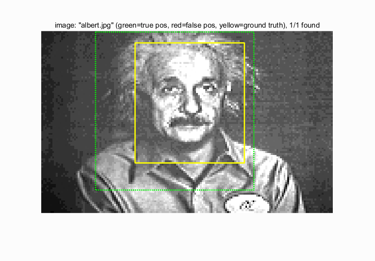
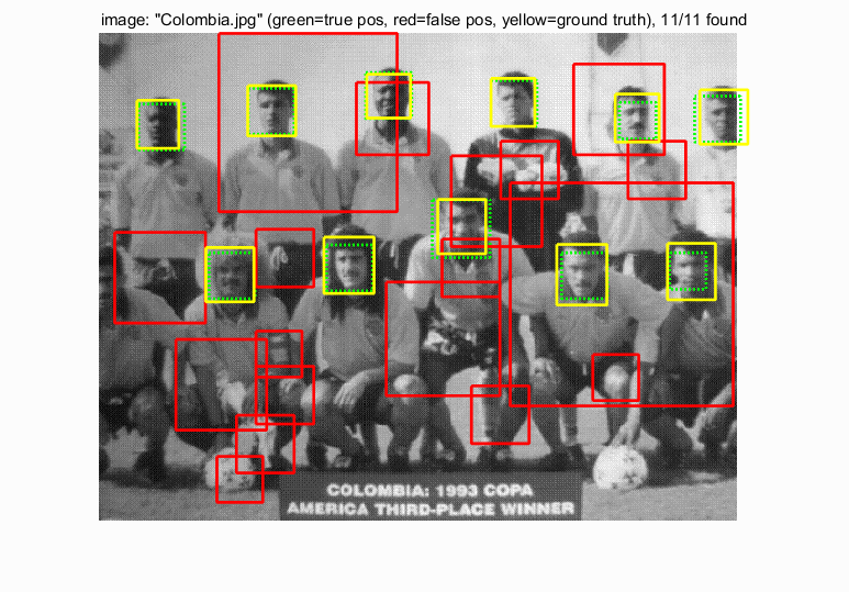
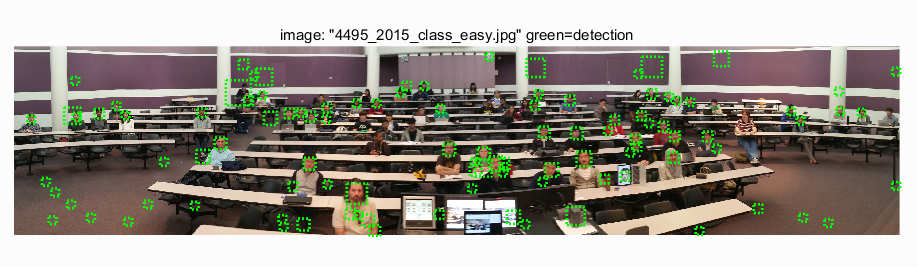
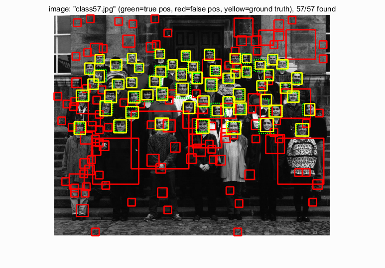
Results for extra scences

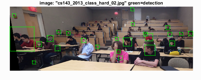
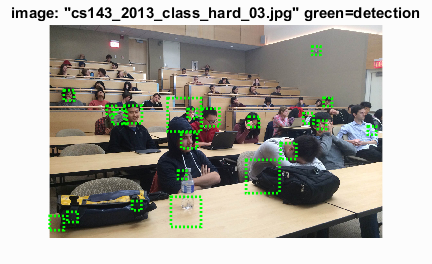
The followings are some results for detecting faces on extra scences with hard mining. Most faces are detected while a high persent of false positives exists:
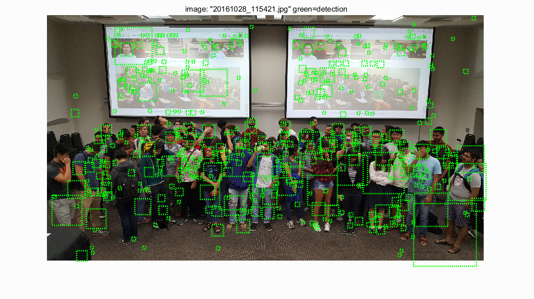
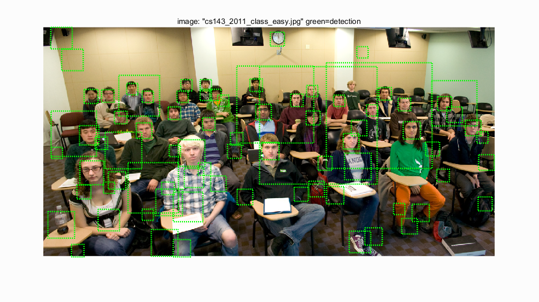
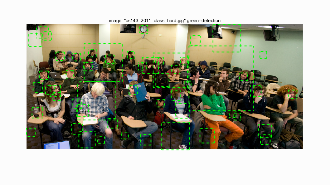