Yuxiang Liu 903109360

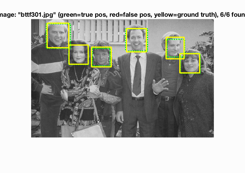
detections_bttf301.jpg

Part I: Get Positive Features

Extract HOG features by calling vl_hog with the given cell size.

Example of code with highlighting

image_files = dir( fullfile( train_path_pos, '*.jpg') ); %Caltech Faces stored as .jpg
num_images = length(image_files);

template_dim = (feature_params.template_size / feature_params.hog_cell_size)^2 * 31;
features_pos = [];
for i = 1:num_images
    img = single(imread(fullfile(train_path_pos, image_files(i).name)));
    img = img/255;
    hog = vl_hog(img, feature_params.hog_cell_size);
    features_pos = [features_pos; reshape(hog,[1,template_dim])];
end

Part II: Get Random Negative Features

First apply sliding window to get image patches, and then extract HOG features using vl_hog, which is similar the Part I.

Example of code with highlighting

image_files = dir( fullfile( non_face_scn_path, '*.jpg' ));
num_images = length(image_files);

template_dim = (feature_params.template_size / feature_params.hog_cell_size)^2 * 31;
features_neg = [];
features_per_img = ceil((num_samples/num_images));

for i = 1:num_images
    img = single(rgb2gray(imread(fullfile(non_face_scn_path,image_files(i).name))));
    [m, n] = size(img);
    for feature_id = 1:features_per_img
        x = ceil((n - feature_params.template_size)*rand());
        y = ceil((m - feature_params.template_size)*rand());
        seg = img(y:y+feature_params.template_size-1,x:x+feature_params.template_size-1);
        hog = vl_hog(seg, feature_params.hog_cell_size);
        features_neg = [features_neg; reshape(hog, [1, template_dim])];
    end
end

Part III: Train SVM classifier

As we did in previous project, call vl_svmtrain to train a linear SVM classifier.

Example of code with highlighting

lambda = 0.0001;
training_data = [features_pos; features_neg]';
num_pos = size(features_pos, 1);
num_neg = size(features_neg, 1);
training_label = [ones(num_pos, 1);-1*ones(num_neg, 1)];
[w, b] = vl_svmtrain(training_data, training_label, lambda);

Part IV: Run Detector

Here's how a multi-scale detector works.(a)Resize the image, and get HOG feature for the whole image. (b)Apply sliding window to get the HOG feature of an image patch. (c)Calculate the confidence of the patch, and keep it if greater than certain threshold.(d)Repeat from step (a)

Example of code with highlighting

test_scenes = dir( fullfile( test_scn_path, '*.jpg' ));

%initialize these as empty and incrementally expand them.
bboxes = zeros(0,4);
confidences = zeros(0,1);
image_ids = cell(0,1);

cell_size = feature_params.hog_cell_size;
tmp_size = feature_params.template_size;
threshold = -0.1;
scale_factor = 0.9;
range = 0:20;
scales = scale_factor .^ range;

for i = 1:length(test_scenes)
      
    fprintf('Detecting faces in %s\n', test_scenes(i).name)
    img = imread( fullfile( test_scn_path, test_scenes(i).name ));
    img = single(img)/255;
    if(size(img,3) > 1)
        img = rgb2gray(img);
    end
    
    cur_bboxes = [];
    cur_confidences =[];
    cur_image_ids = {};
    
    for scale_id = 1:length(scales)
        scale = scales(scale_id);
        scale_img = imresize(img, scale);
        img_hog = vl_hog(scale_img, cell_size);
        [m, n, ~] = size(img_hog);
        for y = 1:(m - tmp_size/cell_size + 1)
            for x = 1:(n - tmp_size/cell_size + 1)
                seg = reshape(img_hog(y:(y + tmp_size/cell_size - 1),...
                    x:(x + tmp_size/cell_size - 1), :), 1, []);
                score = seg * w + b;
                if score > threshold
                    cur_bboxes = [cur_bboxes; ...
                        round([(x-1)*cell_size+1,...
                         (y-1)*cell_size+1,...
                         (x+tmp_size/cell_size-1)*cell_size,...
                         (y+tmp_size/cell_size-1)*cell_size]/scale)];
                    cur_confidences = [cur_confidences; score];
                    cur_image_ids = [cur_image_ids; {test_scenes(i).name}];
                end
            end
        end
    end
    
    if size(cur_bboxes,1)<1
        continue;
    end
    
    [is_maximum] = non_max_supr_bbox(cur_bboxes, cur_confidences, size(img));

    cur_confidences = cur_confidences(is_maximum,:);
    cur_bboxes      = cur_bboxes(     is_maximum,:);
    cur_image_ids   = cur_image_ids(  is_maximum,:);
 
    bboxes      = [bboxes;      cur_bboxes];
    confidences = [confidences; cur_confidences];
    image_ids   = [image_ids;   cur_image_ids];

Results in a table

Here are the results of a baseline detector.
template_size: 36
hog_cell_size: 6
num_negative_examples: 10000
scale_factor: 0.9
times_of_scale: 20
threshold: -0.1
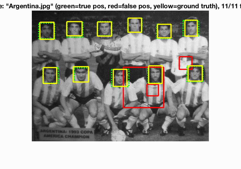
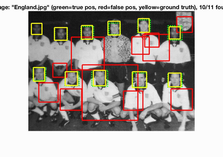
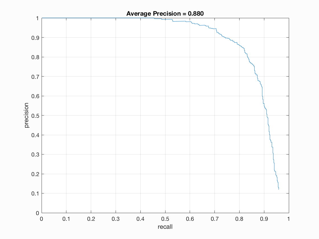
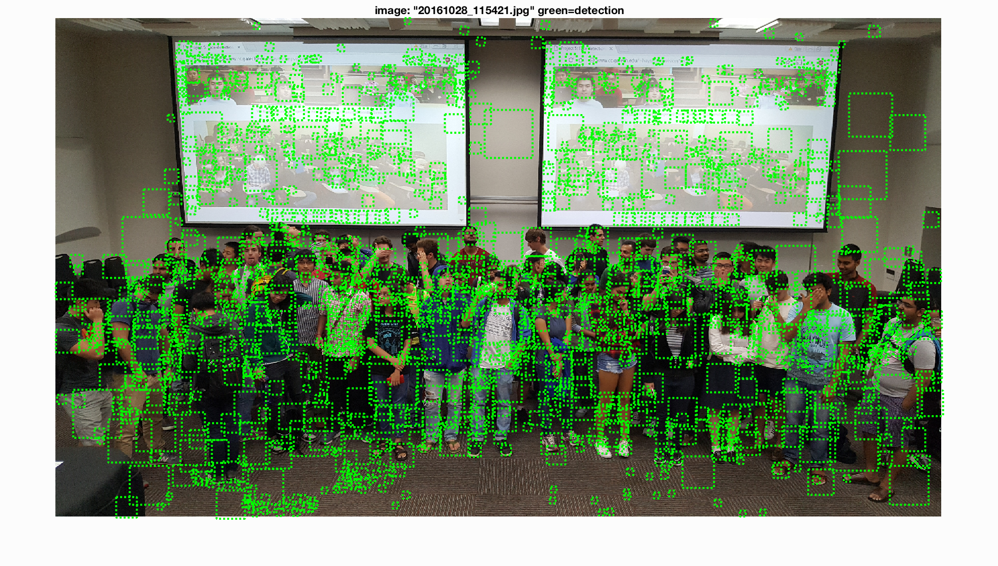
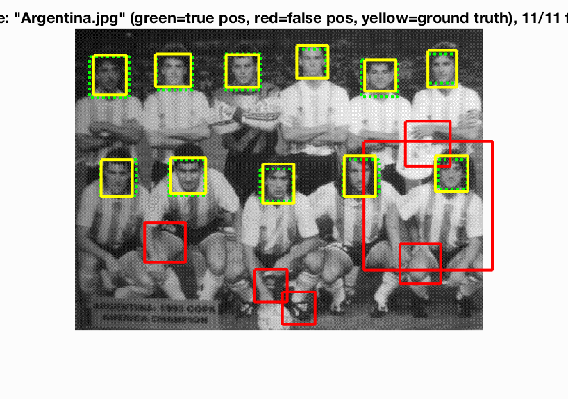
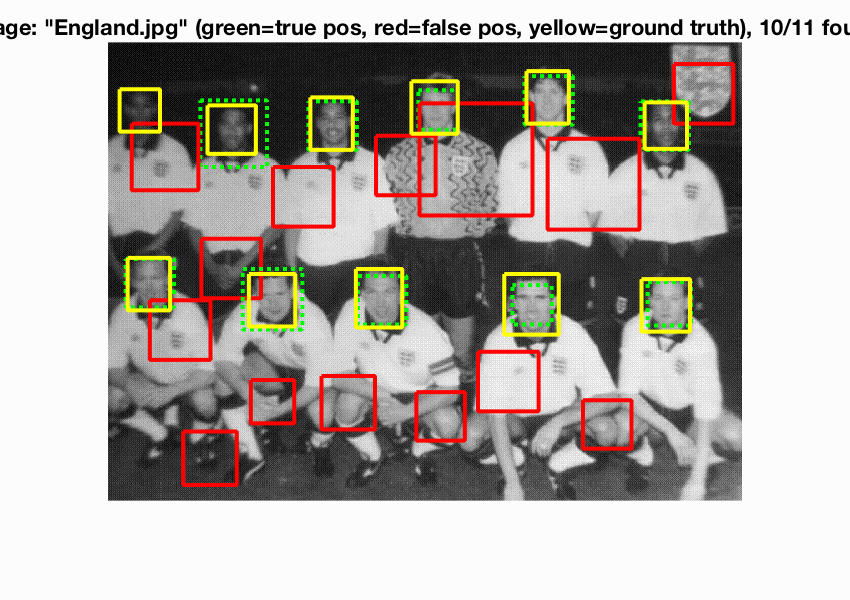
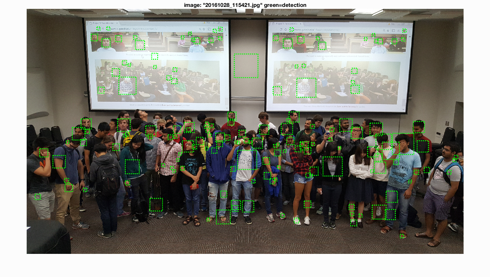
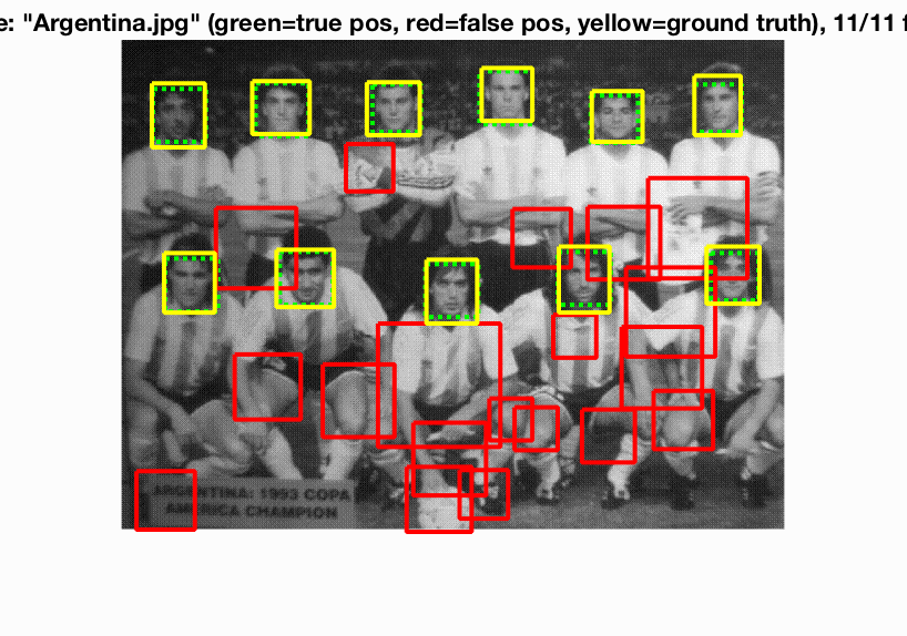
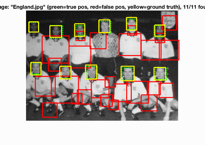
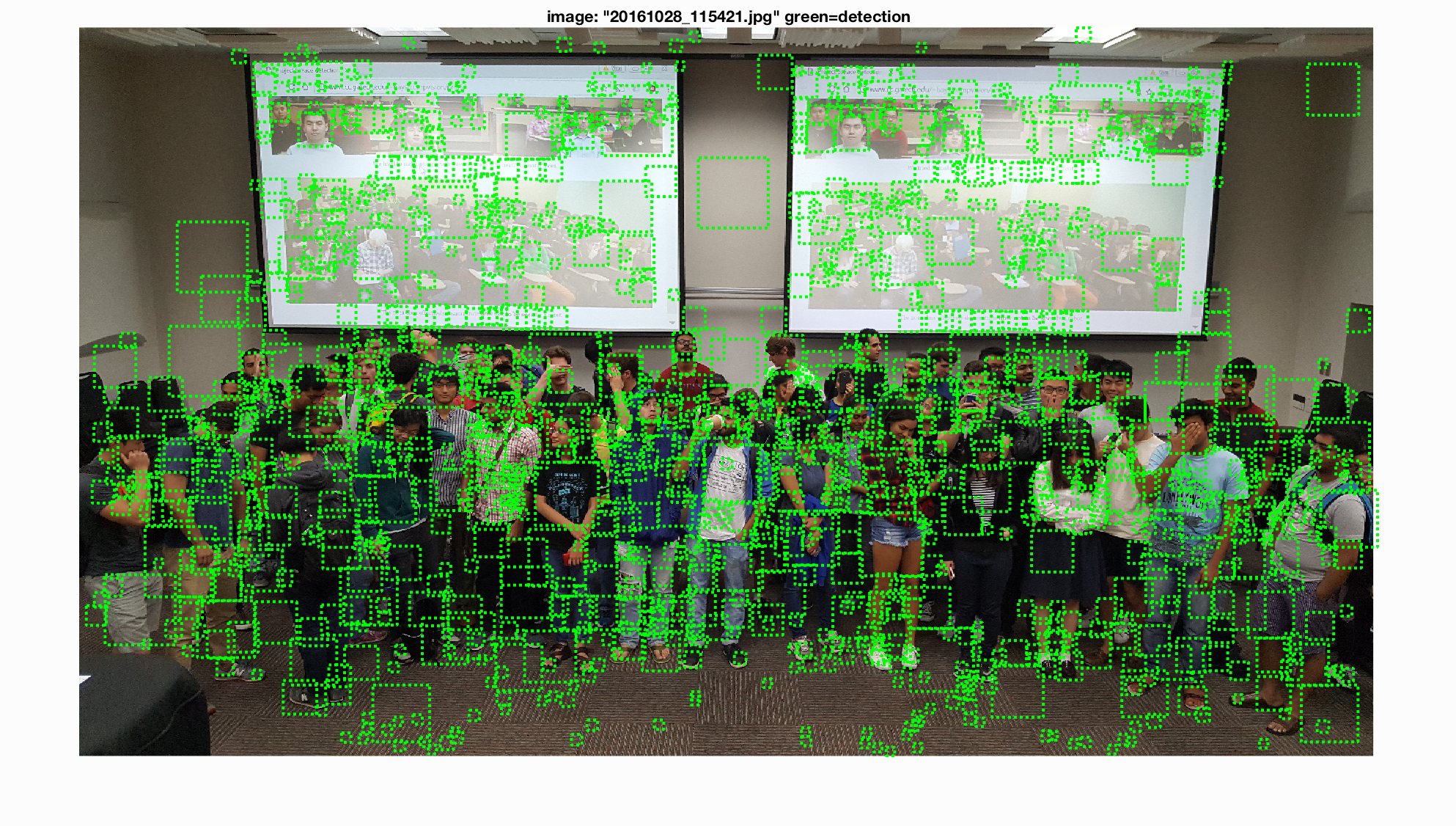
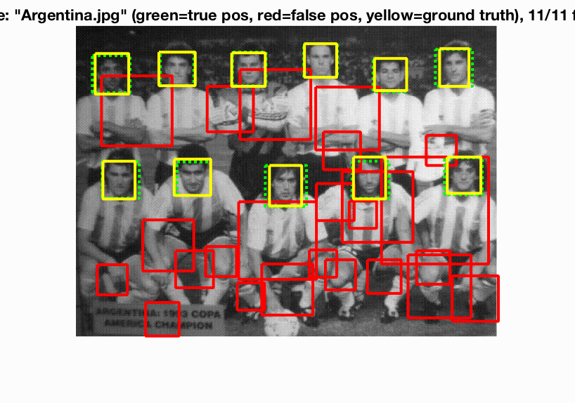
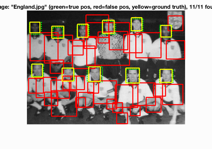
The average precision is 0.880. We can see most faces are detected in the test scenes provided. I also use my detector to test the extra test scenes, and though most faces are detected, the false positive is rather high, which may be caused by my conservative threshold.

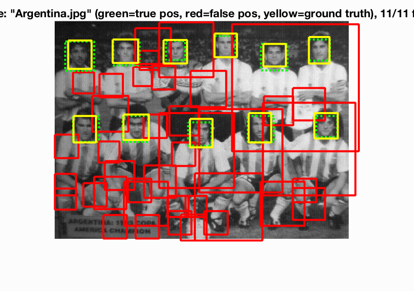
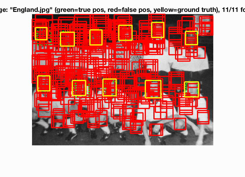
Due to the high false positive, I increase the threshold to 0.9. We can observe that though the average precision decreases slightly, the false positive decreases dramatically, and the final detection picture looks much cleaner!

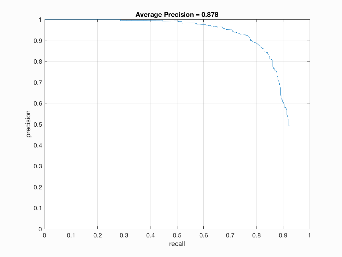
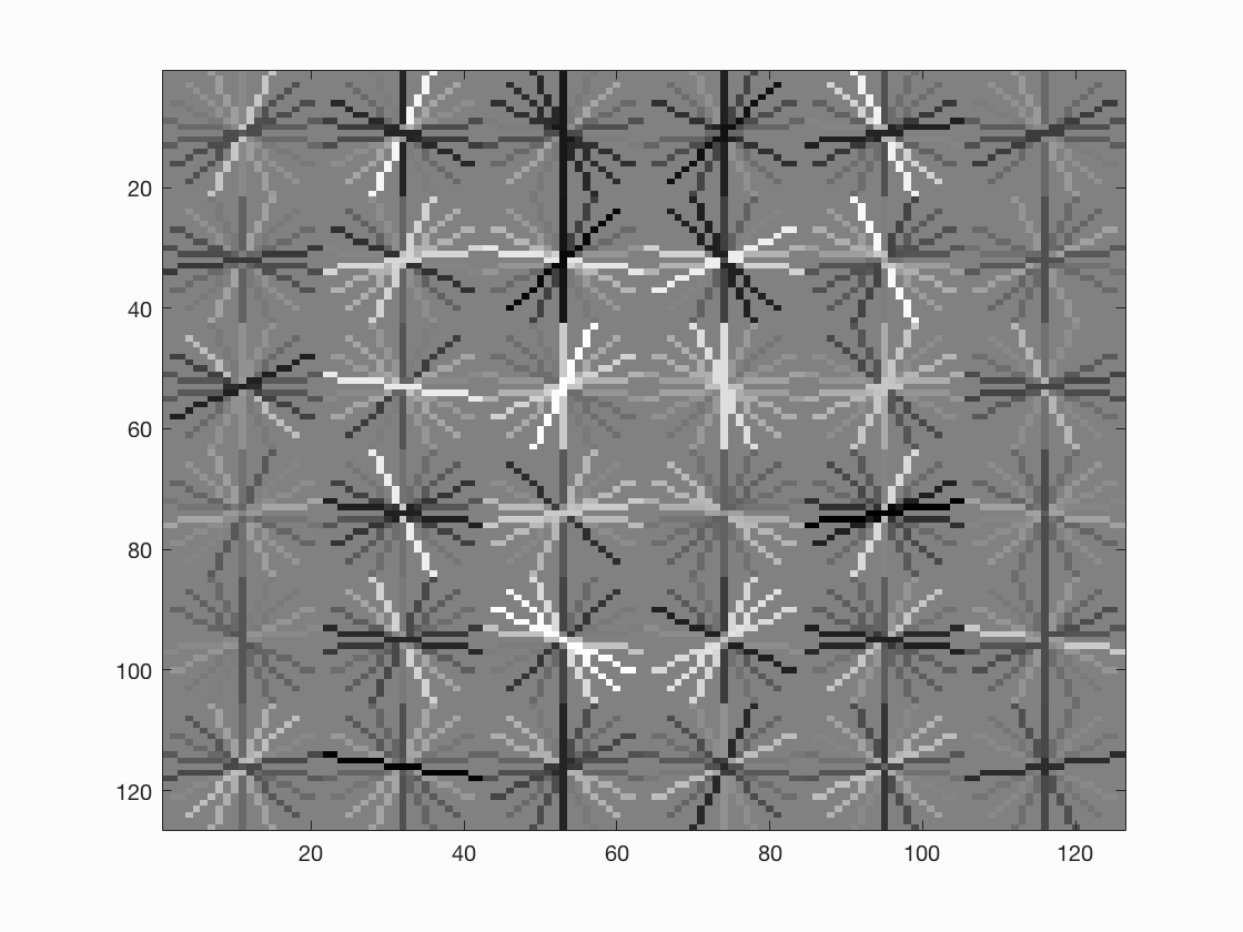
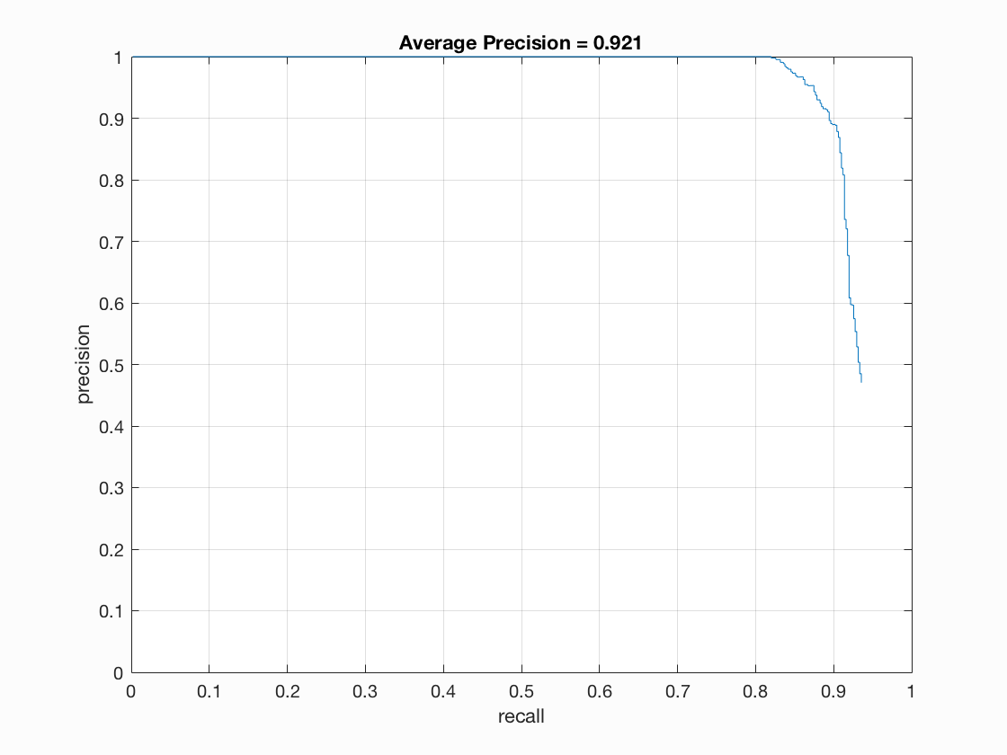
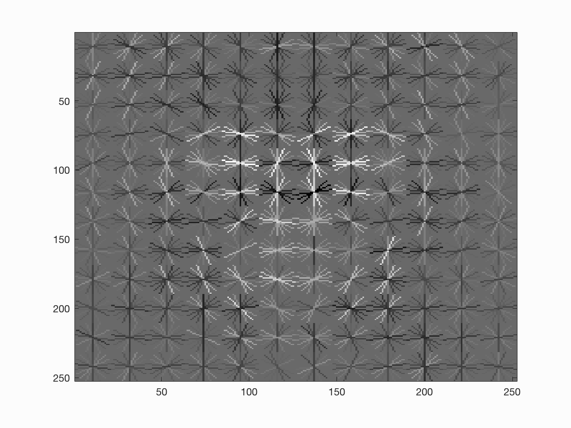
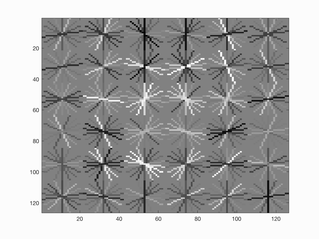
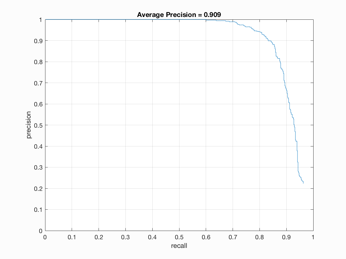
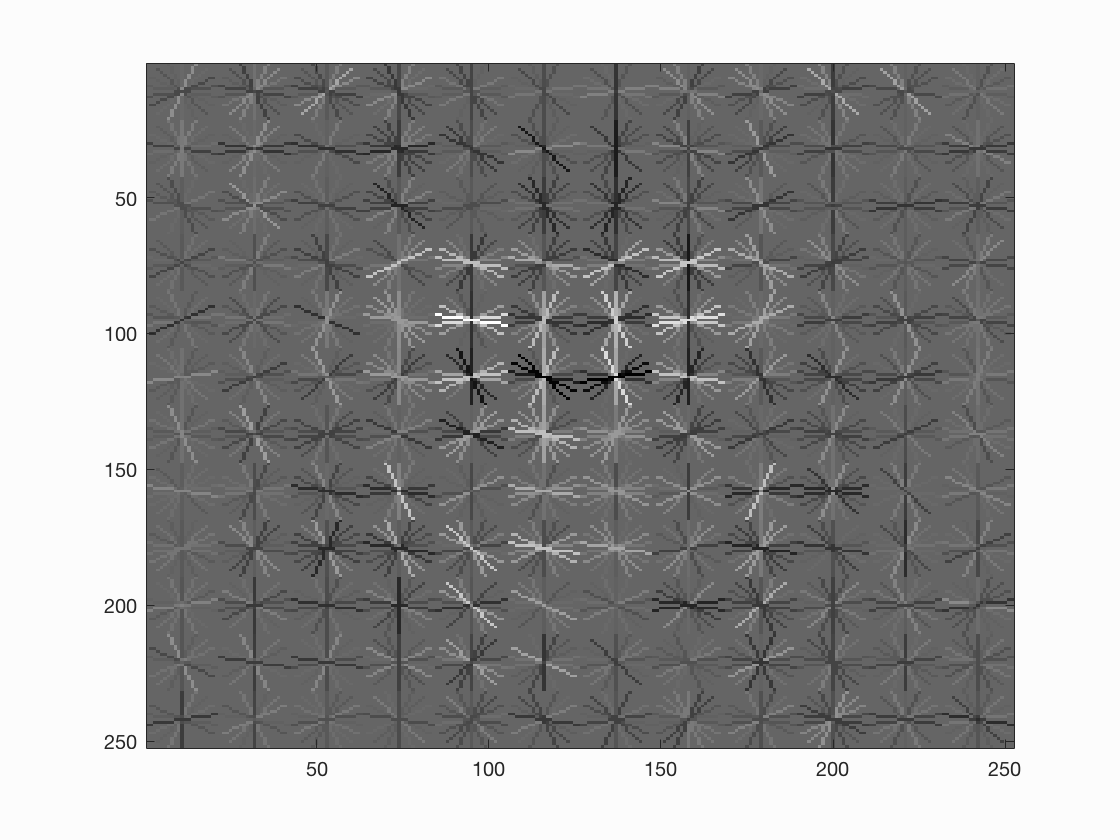
As suggested in the instructions, a smaller cell size may help improve the overall performance. So I set the cell size to be 4, and we can see the average precision increases to 0.909 and the hog template looks better.

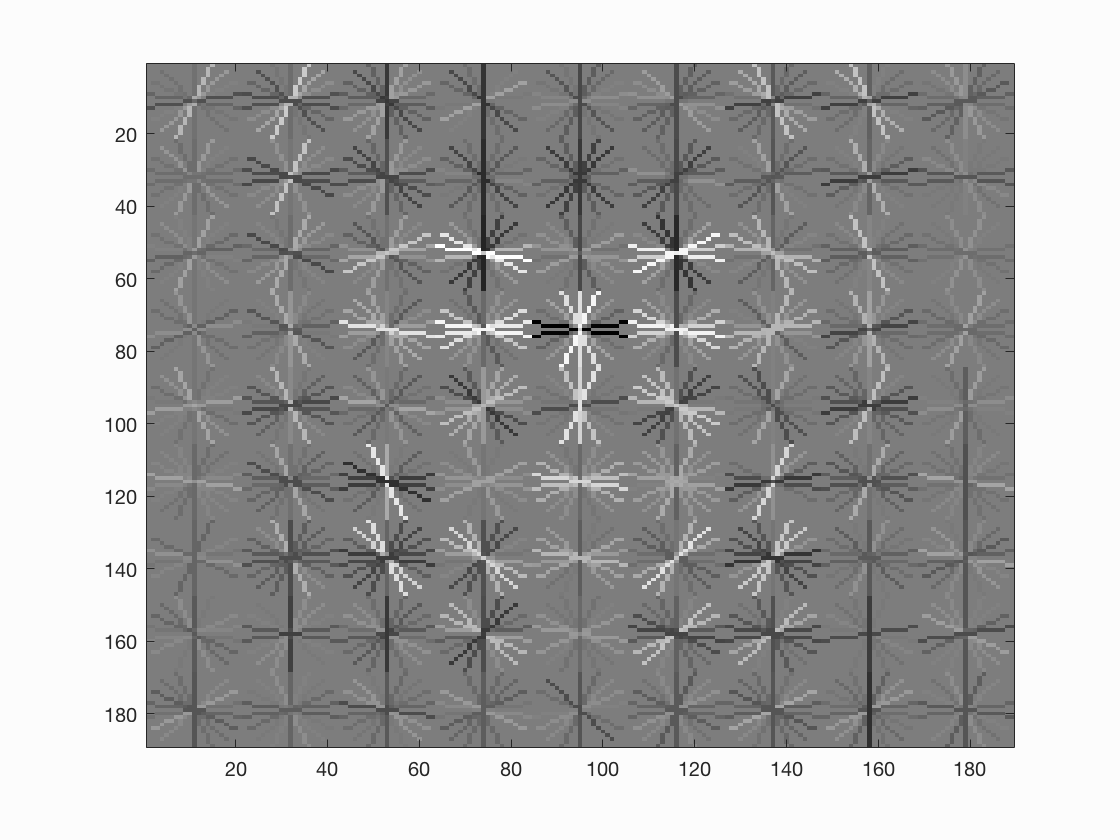
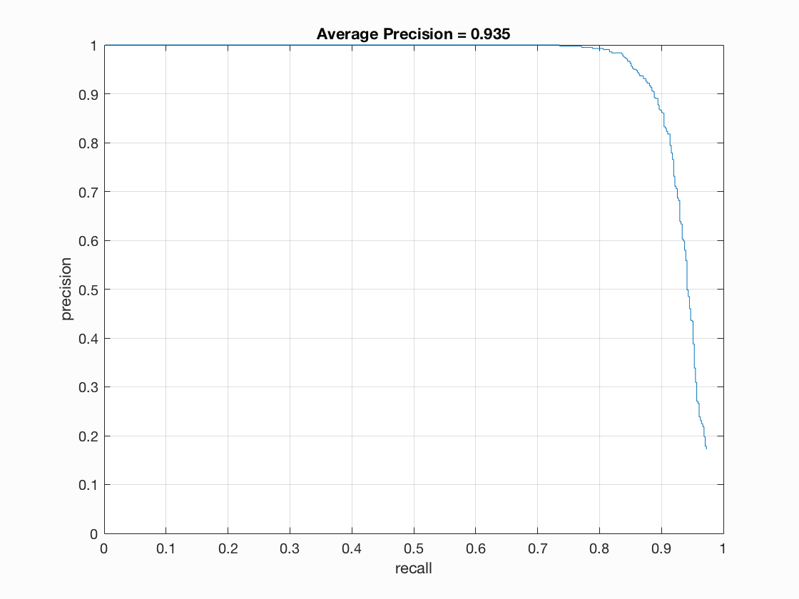
If we further set the cell size to 3, we can see even better average precision with 0.935 and a much better hog template, yet rendering much longer running time.

Extra credit

Hard negative mining
The underlying technique of hard negative mining is that we apply our linear svm classifier on negative images, and then add hard negative features back to our training set again. From the result, we can see the average precision does not increase, yet the false positive decreases remarkably. It makes sense because hard negative mining is equivalent to using more negative samples as training data, thus giving the classifier more power on distinguishing between faces and non-faces.