Zhewei Sun

Implementation Details

For our positive face data, we use a subset of data from the Caltech Web Faces project. Our data set contains 6,713 upright, frontal faces at 36x36 resolution each. The training data is obtained by computing the HoG feature of these images. For the negative data, we extract random 36x36 image patches from a set of non-face images. To ensure variety in our data, the algorithm is configured to extract a uniform number of non-overlapping patches from each image. Once we have the image patches, we can compute their respective HoG features to obtain our training data. The final implementation uses a pixel cell size of 3 for the HoG features and 100,000 random negative examples.

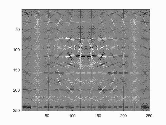
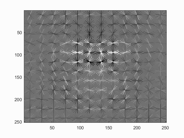
Once we have our training data, we train a linear SVM with a lambda parameter of 0.001. The trained SVM always have virtually perfect accuracy, thus a linear SVM suffices for our task. Below are visualizations of the learned detector.

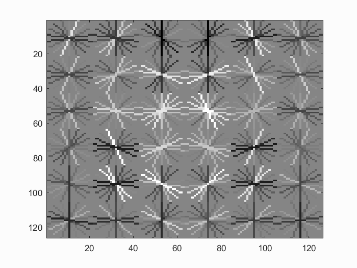
Visualizations of the learned detector using a HoG cell size or 6 and 3 respectively. The visualization with a step size of 3 is the final detector used in this implementation.

Finally, we use a sliding window detector that steps through 36x36 blocks with a step size equivalent to the HoG cell size. For each block, we compute its HoG feature and use the SVM classifier to determine whether it is a face. Once all the blocks are classified, we perform non-maximum suppression on all the bounding boxes found to retrieve the local maximas. Using a single scale detector with a confidence threshold of -0.5, HoG cell size of 6, lambda value of 0.0001, and 10,000 random negative examples, we obtain an average precision of 0.390.

To detect faces at multiple scales, we modify the detector to run over the same image over multiple resolutions. The detector iteratively downsamples the image until it is too small to contain a 36x36 patch. To avoid additive noise, each lower-scaled image is downsampled directly from the original image. Using a step size of 0.7 over scales, the average precision improved to 0.852.

In this implementation, a finer scale step size such as 0.9 does not improve accuracy. In fact, it finds many more false positives and gives a much lower precision. A finer HoG cell step size does help however. By reducing the cell step size from 6 to 3, the accuracy improved to 0.917.

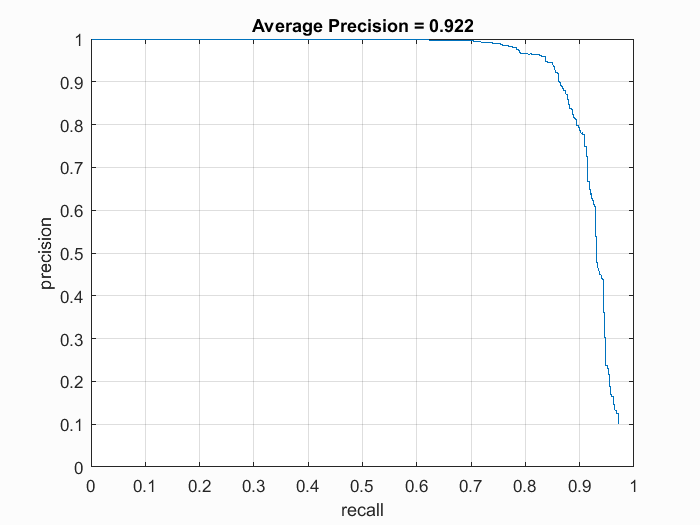
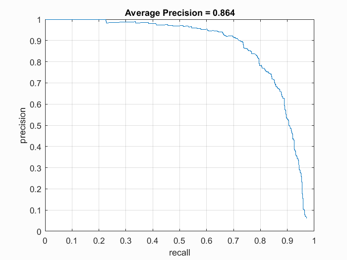
Finally, we tune the parameters further and found that a lambda value of 0.001, cell and scale step sizes of 3 and 0.7 respectively, along with 100,000 random negative examples give us the best results. Using a confidence threshold of -1.0, The detector achieves an average precision of 0.931 in this set-up.

Final results of the face detector.

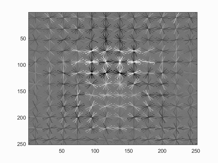
We also tried the hard negative mining technique discussed in Dalal-Triggs. The hard negatives are mined after we train the initial linear SVM, where we run the sliding window detector on the non-face training images without non-maximal suppression. Then, we take the HoG features of all positive classifications as our pool of hard negative examples. We append these new negative examples to our training set and retrain the SVM classifier.

In terms of result, this technique did not improve the average precision. Using the same set of parameters as before, we obtain an average precision of 0.922, as shown below. Although the precision is very similar to the base line, it does reduces the number of false positives by quite a bit, given the same confidence threshold.

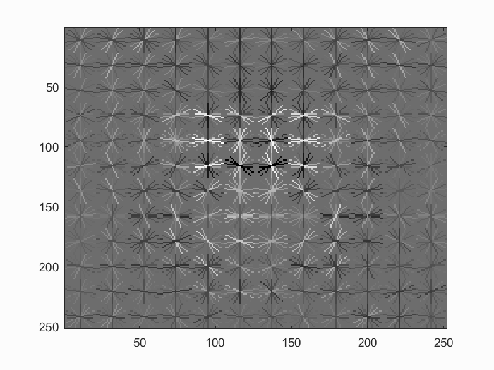
Results using hard negative mining.

Detector learned after hard negative mining

This implementation also includes a self-implemented HoG descriptor. It is implemented as a 36-dimensional feature scheme described by Dalal-Triggs. We first compute the gradient of the given image using central differencing, as suggested by Dalal-Triggs. Then we divide the image into cells and quantize pixels in each cell into an orientation histogram. Each histogram contains 9 bins divided uniformly by unsigned angles between 0 and 180 degrees. We also use bilinear interpolation to combat information losses in quantization. Finally, we perform 2x2 block quantization on the histograms where each cell is normalized with respect to 4 different blocks. Each normalized vector is then concatenated with each other to form a 36 dimensional feature vector.

We verify the correctness of our own HoG feature by comparing it to the vlfeat implementation with 'DalalTriggs' variant. As shown below, both implementations give similar results. It is also worth noting that the UoCTTI variant of HoG does perform much better.

Results of 36-dimensional HoG features using the same parameters from the self-implemented feature and vlfeat's feature. The self-implemented descriptor gives very similar output as the vlfeat implementation. Note that the HoG figures are actually very similar, but the two implementation binned the angles in different orders.

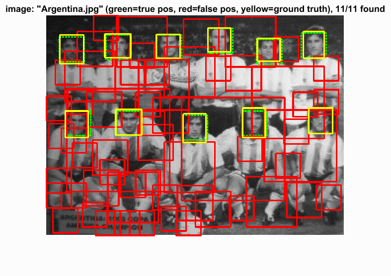
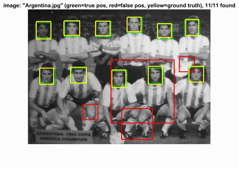
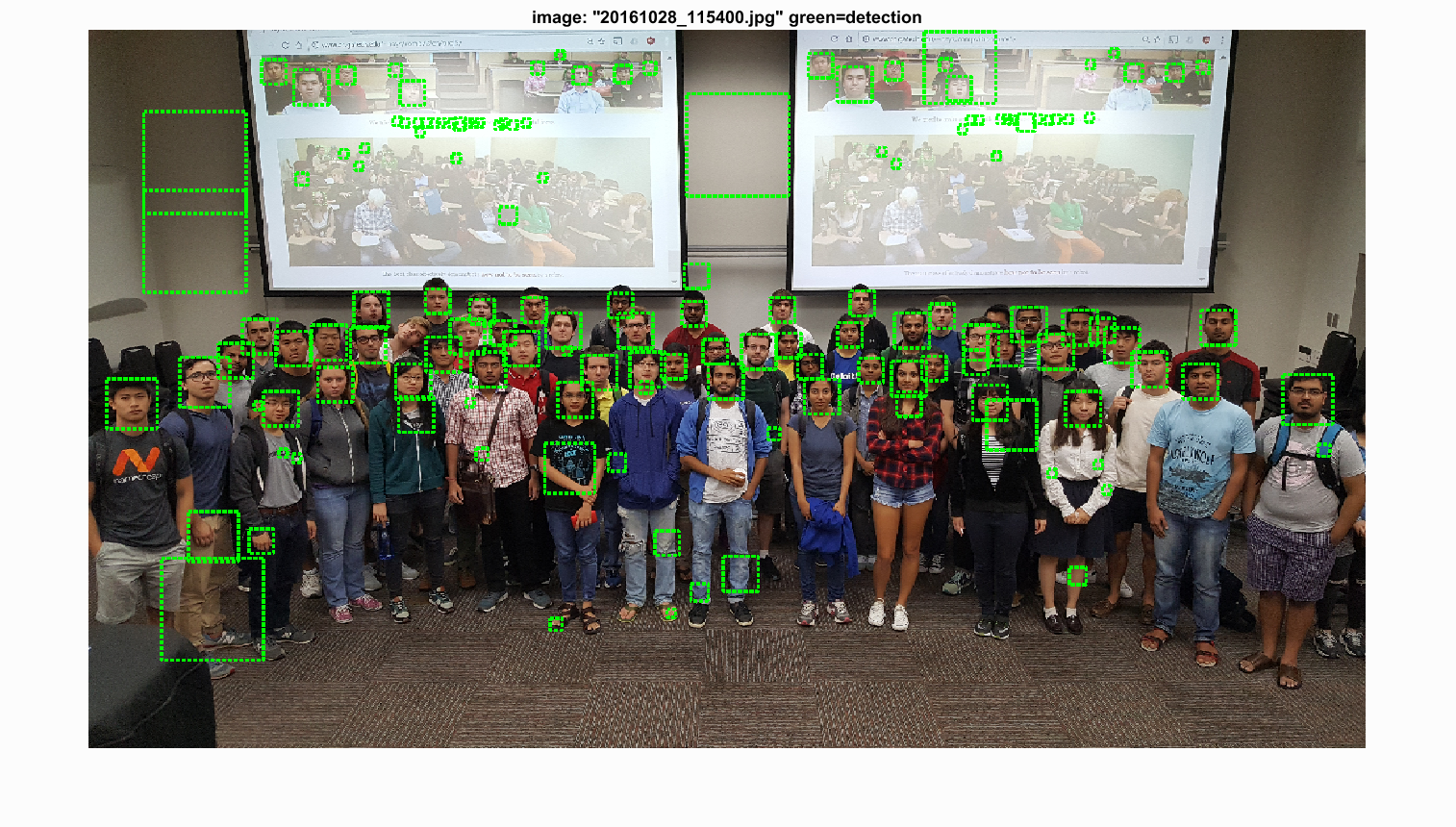
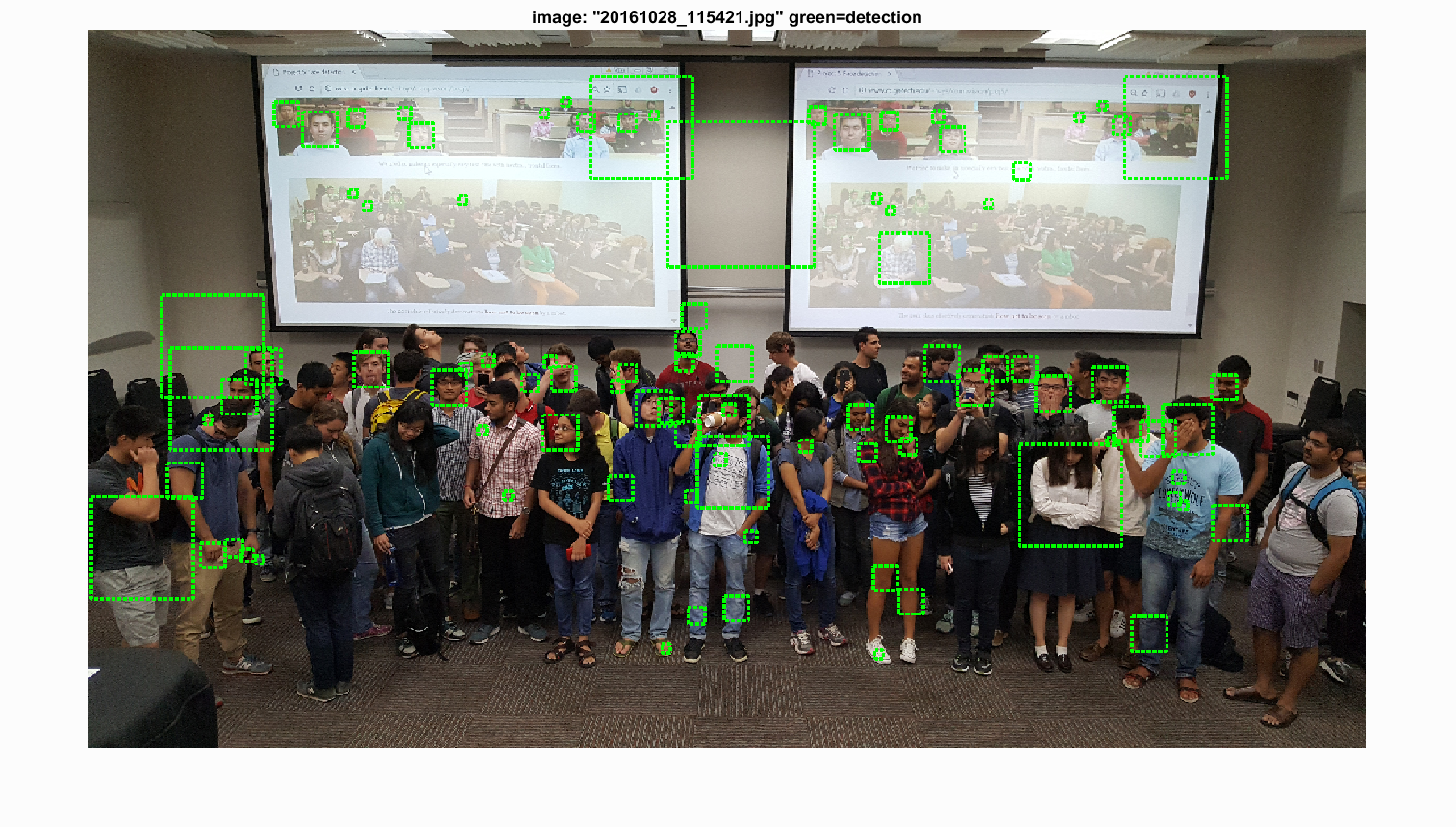
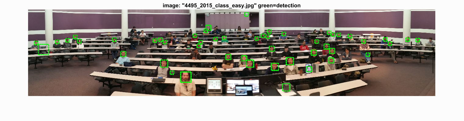
Results on Class Images

Below we present some results from the classroom images. We use the detector with hard negative mining using the same parameters from the previous part.

F2016 CS6476 Class Image - Easy

F2016 CS6476 Class Image - Hard

As we can see, the detector performs fairly well on the easy case where it found almost all the faces (except this one person who tilted his head). It is interesting to note that it also found most of the faces in the easy image on the projector screen. In the hard test case, the face detector misses most of the faces.

Here's a couple more test images:

List of extra credits implemented

- Hard Negative Mining

- HoG Descriptor