Web Resources
1. Introduction
Head tracking is an important processing step for many vision-driven interactive
user interfaces. The obtained position and orientation allow for pose determination
and recognition of simple gestures such as nodding and head shaking. The
stabilized image obtained by perspective de-warping of the facial image
according to the acquired parameters is ideal for facial expression recognition
[3]
or face recognition applications.
We describe the use of a three-dimensional textured model of the human
head under perspective projection to track a person's face. The system
is hand-initialized by projecting an image of the face onto a polygonal
head model. Tracking is achieved by finding the six translation and rotation
parameters to register the rendered images of the textured model with the
video images. We find the parameters by mapping the derivative of the error
with respect to the parameters to intensity gradients in the image. We
use a robust estimator to pool the information and do gradient descent
to find an error minimum.
We implemented a sequential version of the method as well as a parallelized
version which runs on a workstation cluster.
2. The Theoretical Background
We use a 3D-textured polygon model that is matched with the incoming video
stream. We merge graphics and vision by using graphics hardware to produce
renderings that are good enough to match the real images. The initialized
and textured head model is rendered. The intensity difference between rendered
image and video image, in conjunction with the image gradient, is then
mapped to derivatives of our six model parameters. They lead to a local
error minimum that is the best possible match between the rigidly transformed
model and the real video image. The technique can be seen as a more sophisticated
regularization of optical flow, in principle similar to [1].
An additional important feature is the exploitation of graphics hardware.
While special vision hardware such as user-programmable DSPs are still
expensive and not present in an ordinary PC, graphics hardware is ubiquitous
and can be used to render models and to perform hidden surface elimination.
2.1 Mapping Model Parameters to the Image Gradient
Let p be a set of 3D model points with an associated intensity M(p),
and let I(x) be a camera picture. Then using a transformation
T from some model point to screen coordinates with a parameter set {αi},
we minimize the sum over a robust error norm:
 , ,
where ρ is the Geman & McClure robust error norm [5]
defined as
 . .
Here, σ controls the distance beyond which a measurement is
considered an outlier [1].
The error function derived with respect to a particular parameter αj
is
 , ,
where ψ designates the derivative of ρ. Expanding the
second term to evaluate it as a linear combination of the image intensity
gradients we get
 . .
The first factors of the terms are just the image intensity gradient
at the position T(p,{αi}) in the x and
y directions, written as Ix and Iy:
 . .
We use the Sobel operator to determine the intensity gradient at a
point in the image. Note that in this formulation the 3D model, its parameterization,
and the 3D to 2D transformation used are arbitrary provided the model can
be rendered onto the screen.
2.2 Special Case: Rigid Transformation and Perspective Projection
For our more specific case we use the transformation matrix, written in
homogenous coordinates, going from 3D to 2D:
 , ,
with Rx, Ry, and Rz
being rotation matrices around the x, y, and z axis,
for some angles rx, ry, and rz
respectively. tx, ty, and tz
are translations along the axes. We assume that the focal length f
is known and found that a rough estimate gives good results. Without loss
of generality, we assume that rx = ry = rz =
tx = ty = tz = 0, which corresponds to
a camera at the origin looking down the positive z-axis. Note that in this
case the order of rotations does not affect our calculations.
Omitting the parameters of I,
Ix, and Iy,
we obtain as derivatives of the intensity with respect to our parameters
for a particular model point p = (px,
py,
pz)T
 , ,
 , ,
 , ,
 , ,
 , ,
 . .
For color video footage we use the Geman & McClure norm on the
distance in RGB space rather than on each color channel separately. σ
is set such that anything beyond a color distance of 50 within the 2563
color cube is considered an outlier. We sum the results of each color channel
to obtain a minimum error estimate.
2.3 Model Parameterization with Uncorrelated Feature Sets
 The
parameterization given above is not adequate for implementation because
the rotations and translations of the camera used in the parameterization
look very similar in the camera view resulting in correlated feature sets.
For example, rotating around the y-axis looks similar to translating
along the x-axis. In both cases the image content slides horizontally,
with slight differences in perspective distortion. In the error function
space this results in long, narrow valleys with a very small gradient along
the bottom of the valley. It destabilizes and slows down any gradient-based
minimization technique. The
parameterization given above is not adequate for implementation because
the rotations and translations of the camera used in the parameterization
look very similar in the camera view resulting in correlated feature sets.
For example, rotating around the y-axis looks similar to translating
along the x-axis. In both cases the image content slides horizontally,
with slight differences in perspective distortion. In the error function
space this results in long, narrow valleys with a very small gradient along
the bottom of the valley. It destabilizes and slows down any gradient-based
minimization technique.
A similar problem is translation along and rotation around the z-axis,
which causes the image of the head not only to change size or to rotate,
but also to translate if the head is not exactly in the screen center.
To overcome these problems we choose different parameters for our implementation
than those given in 2.2. They are illustrated in the figure on the right.
We again assume that the camera is at the origin, looking along positive
z, and that the object is at some point (ox, oy,
oz).
Note that the directions of the rotation axes depend on the position
of the head. rcx and rcy have the same
axis as rox and roy, respectively,
but rotate around the camera as opposed to around the object.
rcx
and rox are orthogonal to both the connecting line between
the camera and the head, and to the screen's vertical axis. Rotation around
rcx
causes the head image to move vertically on the screen, but it is not rotating
relative to the viewer and it does not change its horizontal position.
Rotation around
rox causes the head to tilt up and down,
but keeps its screen position unchanged.
rcy and roy are defined similarly
for the screen's horizontal coordinate. Note that rcy/roy
and rcx/rox are not orthogonal except
when the object is on the optical axis. However, the pixel movement on
the screen that is caused by rotation around them is always orthogonal.
It is vertical for the rcy/roy pair
and horizontal for the rcx/rox pair.
Rotation around rco causes the head's image to rotate
around itself, while translation along
tco varies the
size of the image. Neither changes the head screen position.
The parameterization depends on the current model position and changes
while the algorithm converges. Different axes of rotation and translation
are used for each iteration step.
We now have to find the derivatives of the error function with respect
to our new parameter set. Fortunately, in Euclidean space any complex rotational
movement is a combination of rotation around the origin and translation.
We have already calculated the derivatives for both in section 2.2. The
derivatives of our new parameter set are linear combinations of the derivatives
of the naïve parameter set.
The parameterization change does not eliminate the long valleys we
started with. Instead, they are now oriented along the principal axes of
the error function space. Simple parameter scaling can convert the narrow
valleys to more circular-shaped bowls; these allow for efficient nonlinear
minimization. In 2D subspace plots of the error function we visually inspect
the shape of the minimum and adjust the scaling appropriately.
For convergence we use simple steepest descent. While more sophisticated
schemes like conjugate gradients brought relatively large improvements
to the naïve parameterization, we did not see any improvements with our
final model. One reason is certainly that our error function is discretely
defined and possibly far from quadratic. Additionally, the Hessian matrix
may rapidly change during the iterations.
Our a priori efforts to find good parameters and suitable scales exploit
the underlying structure of the problem and are crucial for speeding up
convergence.
2.4 Relationship between Uncorrelated Feature Sets and Preconditioning
Using uncorrelated features is equivalent to making the Hessian matrix,
the second derivative of the error function, almost diagonal near the error
function minimum. Choosing an appropriate scale for each of the parameters
brings the condition number of the Hessian matrix close to unity, which
is the goal of preconditioning in a general nonlinear minimizer. In our
case we use a priori knowledge to avoid any analysis of the error function
during run-time.
3. Implementation Features
The sequential and the parallel implementation share common features that
are now described. They both use Gaussian pyramids to deal with large head
motions and OpenGL to perform visible surface determination and rendering
of the textured model.
3.1 Gaussian Pyramid
To allow larger head motions, a 2-level Gaussian pyramid is used. For each
frame, the parameters are optimized at a resolution of 40 x 30 pixels,
and the optimized parameters are taken as the starting point to optimize
at the 80 x 60 pixels resolution. For video footage where the head covers
a large part of the screen the rather small resolution of 80 x 60 is sufficient
for good parameter extraction. Higher resolutions do not give better results.
Details that are only visible at higher resolutions are unlikely to be
matched exactly due to the inaccuracy of our head model. Matching those
model errors does not improve the accuracy of the extracted parameters.
3.2 Using OpenGL
Our model is a male head from Viewpoint Data Labs of 7000 triangles that
was reduced to 500 triangles. The model is taken as is and is not customized
to the test user's head. For each evaluation of the derivatives, two OpenGL
renderings of the head are performed. The first rendering is for obtaining
the textured image of the head using trilinear mipmapping to cope with
varying resolution levels and head distances to the camera.
The second rendering provides flat-filled aliased polygons. Each polygon
has a different color for visible surface determination in hardware. By
walking through the image and identifying the polygon that is found at
the current pixel position the 2D screen coordinates can be converted back
into 3D model coordinates. All transformations into camera and screen coordinates
and the calculations of gradients to compute the parameter derivatives
are done only for visible surfaces.
Note that for our application, aliasing during the rendering step that
determines the visible polygons is not a problem. Although visible polygons
might be missed because of aliasing, polygon vertex information is only
used to determine the 3D coordinates of a point in the image but nothing
is done to the polygon itself. When initially projecting the texture onto
the model visible surface computation is done at a higher resolution to
reliably texture all visible polygons.
4. The Sequential Implementation
4.1 Implementation Details
In the sequential version minimization of the parameters is done using
nonlinear conjugate gradient with variable step size. Minimization is completed
for the low resolution level, then the result is taken as the starting
point of the higher resolution level where minimization is done again to
find the final parameter set. For each gradient computation in the conjugate
gradient algorithm the model is rendered using the current parameters as
described in 3.2 and the gradient is calculated. Up to 10 gradient evaluations
are needed per level to reach the minimum.
4.2 Results


Figure 1: Large head rotation and translation between two frames.
Top: video image, middle: rendered model, bottom: stabilized image obtained
by reprojection onto the model.
The robustness of the algorithm against large changes in the head parameters
is impressive; rotations of more than 25 degrees and translations of more
than half of the head size from one image to the next still converge. Figures
1 shows one example of rotation and one of translation each showing large
movements between two frames. Note that the test subject wears glasses
and there are specular reflections on the subject's forehead from the ceiling
lights.


Figure 2: The test sequence at 0 s, 2 s, 4 s, 6 s, 8 s and 9 s.
Top: video, middle: model, bottom: stabilized image.
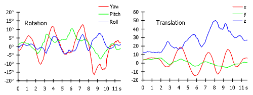
Figure 3: The translation and rotation parameters for the whole sequence.
Our algorithm has problems when no texture data is available or when
the 3D model differs extensively from the actual head geometry of the subject.
We only project a single texture from a frontal view onto the model. The
sides of the model thus remain untextured or are only textured in low resolutions
due to the small angle of incidence. Thus, head rotations where only the
sides remain visible are registered with poor accuracy. Figure 2 shows
images of a test sequence taken at 15 fps. During the first 8 seconds tracking
is stable and the obtained stabilized image is usable. During the ninth
second of the sequence the combination of a large head rotation and an
incorrect registration of a specular reflection in the video with a reflection
on the model lead to incorrect measurements. Figure 5 shows a sudden change
in yaw around the ninth second, which corresponds to the incorrect registration.
In such cases accurate tracking is usually reacquired when the head returns
to a more front-facing orientation.
A major gain in performance can be expected when not only a single
frontal image is used for projection but pictures from the sides as well.
Another improvement would be a customizable head model to more accurately
exploit head surface details such as nose and ear positions.
4.3 Speed and the Impact of OpenGL Acceleration
The sequential implementation runs at 1.7 s/frame using Windows NT's software
OpenGL rendering on a Pentium Pro 200 Mhz machine.
Our tests with OpenGL hardware for rendering are not yet complete.
Using the original 7000 polygon model on a Pentium II 300 MHz an ATI Rage
Pro AGP graphics card that only accelerates pixel operations but not the
geometry was about 20 % faster than Microsoft's OpenGL software implementation
on this computer. With the 500 polygon model on the PentiumPro 200 Mhz
a Diamond FireGL 1000pro PCI that accelerates geometry calculation as well
as pixel operations and that is in general better suited to OpenGL acceleration
than the ATI card was slower than software rendering in main memory.
A significant bottleneck could be copying the frame buffer out of the
graphic card memory into main memory for processing which has to be done
if a graphic accelerator is used. Copying also occurs for the software
implementation since OpenGL does not let the application access its frame
buffer directly but it is done out of main memory in this case. The difference
between AGP and PCI bus systems could be decisive, but further testing
is needed.
In general rapid advances in cheap graphics accelerator technology
can be effectively used to improve the performance of our system. The ratio
of OpenGL rendering time to main processor computation time changes with
model complexity. Generally, similar systems with more complicated models
will benefit more from OpenGL acceleration.
5. The Parallel Implementation
5.1 Implementation Details
To speed up our system and to bring it closer to real time performance
the system was implemented on a 8 node workstation cluster with single
Pentium Pro 200 MHz on each node.
Common parallel implementations of minimization techniques such as
gradient descent rely on partitioning the problem space into subspaces
of smaller dimensionality that are minimized individually on each node
with periodic synchronization between processors. Several variants of this
concept exists, they belong to the class of Parallel Variable Transformation
algorithms [4]. It relies on the assumption that
the computational load is proportional to the number of partial derivatives
computed. However, in our case rendering the model and doing visible surface
detection and screen coordinates to model coordinates transformation has
to be done for any computation of partial derivatives. The computation
of the derivatives themselves is not the major computational burden, and
algorithms based on Parallel Variable Transformation show poor scalability.
Partitioning the image and processing the created tiles on different
processors is possible but not efficient. Geometric computations and clipping
has to be done for every tile. Also communication overhead increases, for
every gradient evaluation messages have to be exchanged with every workstation.
Figure 4: Overview of the parallel implementation.
Instead we took a different approach. We parallelize the system by performing
multiple error and gradient evaluations simultaneously, each one on a separate
cluster node. We evaluate at 7 points spreaded the current position and
fit a quadratic to these data points. The minimum of the quadratic is taken
as the new model parameters. To avoid gross outliers the minimum is restricted
to be within some region around the current parameters using the hook-step
method described in [2]. The process is repeated
with a smaller spread of the data points. These two iterations are done
for each level of the Gaussian pyramid.
The method is extended to be more adaptive to the incoming video stream.
The parameter vectors of the two previous frames are extrapolated to the
current camera frame. If the current head movement is fast, at the first
evaluation step within each camera frame more evaluation points are inserted
between the previous head position and the extrapolated position. The fitting
of the quadratic is done using only the lowest point and its six nearest
neighbors.
5.2 Results
All test sequences were rerun using the new parallel technique. Since the
error function is relatively benign the obtained parameters are nearly
as accurate as those obtained using sequential conjugate gradient. The
method also shows similar stability. The computation is much faster, about
.25 s/frame.
References
-
M. Black and P. Anandan. The robust estimation of multiple motions: parametric
and piecewise-smooth flow fields. TR P93-00104, Xerox PARC, 1993.
-
J. E. Dennis, R. B. Schnabel. Numerical Methods for Unconstrained Optimization
and Nonlinear Equations, ch. 6. Prentice-Hall 1993.
-
I. Essa and A. Pentland. Coding analysis, interpretation, and recognition
of facial expressions. PAMI, 19(7): 757-763, 1997.
-
M. Fukushima. Parallel Variable Transformation in Unconstrained Optimization.
SIAM J. Optim., Vol. 8, No. 4, pp. 658-672, August 1998.
-
S. Geman and D. E. McClure. Statistical methods for tomographic image reconstruction,
Bull. Int. Statist. Inst. LII-4, 5-21, 1987.
|
|
|
| |