We show how to use color graphics to visualize a function of a complex variable or other two dimensional vector fields. A gallery of familiar complex functions as well as some physical applications are displayed demonstrating the use of this technique.
Most of us have some sort of mental image when we are presented with the concepts of a pole, a zero, a branch point or a branch cut. Most graphical techniques for describing complex functions are quite crude in that poles and zeros may be represented by x's and o's and branch cuts identified by thick lines, but detailed phase information is usually lost as well as pole and zero multiplicity data. Here we propose a standard for displaying complex functions that uses color to convey both intensity and phase information.
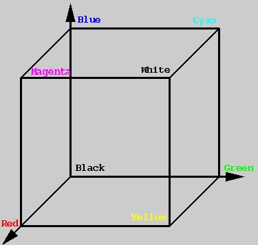
Color space is a compact three dimensional space, and a point in the space can be uniquely specified by the three intensities [r,g,b] that represent the intensity of the Red, Green and Blue electron guns in a color display tube. The intensities r,g and b each lie in the interval [0,1]. The eight vertices of the color cube are shown in Table 1. and are also displayed in Figure 1.
Table 1: The [r,g,b] values for the eight corners of the color cube.
[r,g,b]          Color

[0,0,0]          Black
[1,0,0]          Red
[0,1,0]          Green
[0,0,1]          Blue
[1,1,0]          Yellow
[1,0,1]          Magenta
[0,1,1]          Cyan
[1,1,1]          White
Figure 1: The Color Cube
To visualize a complex number z = x + i y or a two dimensional vector field
[v ,v ]
  1  2
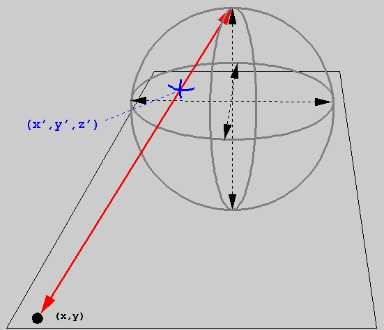
we must find a mapping from C or equivalently R x R into the color cube [0,1] x [0,1] x [0,1]. There are an infinite number of possible mappings to choose from. One well known mapping stereographically maps the complex plane onto the surface of the unit sphere by finding the intersection of the ray that passes through the North pole [0,0,1] and the point in the plane [x,y,0]. Points that lie inside the unit circle in the complex plane are mapped to the southern hemisphere and the origin z=0 is mapped to the South pole [0,0,-1]. Points that lie outside the unit circle are mapped to the northern hemisphere and all points at infinity are mapped to the North pole [0,0,1]. Points on the unit circle map directly to the equator. This mapping is defined by
                             2   2
             [ 2 x , 2 y , x + y + 1 ]
[x',y',z'] = -------------------------
                    2   2
                   x + y + 1
and this projection is shown in Figure 2.
Figure 2: Stereographic projection of the complex plane onto the surface of the unit sphere.
One natural way to imbed the unit sphere in the color cube is by shrinking its radius to 1/2 and placing the center of the sphere at the center of the color cube [r,g,b] =[1/2,1/2,1/2].We align the southern to northern axis of the sphere along the ray from [0,0,0] to [1,1,1] in the color cube. This orientation is chosen so that the South pole is as close to Black [0,0,0] as possible ( aesthetically zeroes which have no amplitude ought to be black ) and the North pole is as close to White [1,1,1] as possible ( likewise poles ought which have enormous amplitudes ought to be white ).
The azimuthal orientation will be uniquely determined if we require that the positive real axis has maximal red intensity ( R is for real or red! ). This map looks quite reasonable on the unit circle but the intensities at the origin and infinity are not distinct enough. This is because a sphere of radius 1/2 can only have points that are a fraction 1/sqrt(3) or about 58% of the distance to the corners at [0,0,0] and [1,1,1] which leads to weak intensities. Intensities for poles are not bright enough and zeros are not dark enough.To remedy this situation we will replace each hemisphere of the sphere by separate cones whose vertices are at [0,0,0] and [1,1,1] andwhose bases lie on the equator.
In a coordinate system where the z axis is the axis of the cones, this mapping is defined by:
        2 x                 2 y
x'= ----------- , y' =  ----------- ,
         2    2              2    2
    1 + x  + y          1 + x  + y

                  2    2           2    2        2    2
    sqrt(3) (1 + x  + y  - 2 sqrt(x  + y )) eta(x  + y - 1 )
z'= --------------------------------------------------------
                                2    2
                           1 + x  + y
,where eta(t) is the sign function defined by:
         { -1     t < 0 }
eta(t) = {  0     t = 0 }  .
         {  1     t > 0 }
If we rescale this mapping by a factor of 1/2, followed by a rotation to align the cones axis with the diagonal of the color cube and follow this by a translation to the center of the color cube we obtain the intensities [r,g,b] as a function of z=x+i y:
    1            1    R        2      x
r = - + eta(R-1)(- - ----) + ------- ----
    2            2      2    sqrt(6)    2
                     1+R             1+R

    1            1    R        1      x       1      y
g = - + eta(R-1)(- - ----) - ------- ---- + ------- ----
    2            2      2    sqrt(6)    2   sqrt(2)    2
                     1+R             1+R            1+R

    1            1    R        1      x       1      y
b = - + eta(R-1)(- - ----) - ------- ---- - ------- ----
    2            2      2    sqrt(6)    2   sqrt(2)    2
                     1+R             1+R            1+R
where
 2   2   2
R = x + y  .
These completely define our mappings from the complex plane into the color cube.This map has the desired properties at poles and zeros and will be explored visually in the next section. Below is a C code fragment that computes this mapping.
C language code fragment for computing color intensities.
double x,y, red,green,blue, a,b,d,r,sqrt();
   r = sqrt(x*x+y*y);
   a = 0.40824829046386301636 * x;
   b = 0.70710678118654752440 * y;
   d = 1.0/(1. + r*r);
   red = 0.5 + 0.81649658092772603273 * x * d;
   green = 0.5 - d * ( a - b );
   blue = 0.5 - d * ( a + b );
   d = 0.5 - r*d;
   if( r < 1 ) d = -d;
   red += d;
   green += d;
   blue += d;
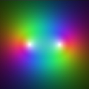
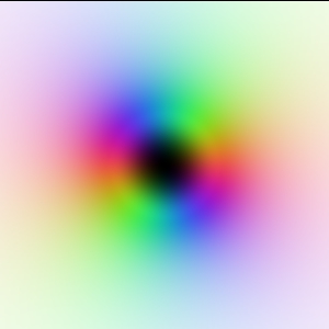
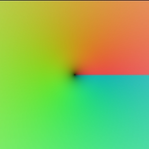
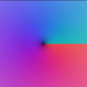
We will visualize a large class of complex functions and describe in some detail their visual properties. We will look at: z, 1/z, z^2, 1/z^2, sqrt(z) in a mathematical sense and 1/(z-1)-1/(z+1), 1/(z-i)-1/(z+i), and 1/(z-1)-1/(z+1) -1/(z-i)+1/(z+i) in a physical sense.
f(z) = z f(z) = 1/z
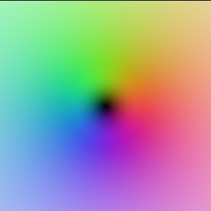
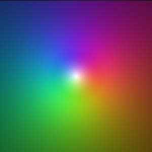
Notice that zeroes are black and poles are white. As one traverses around the unit circle, z and 1/z pass through the colors in the opposite direction. Starting on the real axis and moving counter-clockwise, f(z) = z passes through red -> green -> blue , while f(z) = 1/z passes through the same colors moving in a clockwise direction.
f(z) = z*z f(z) = 1/(z*z)
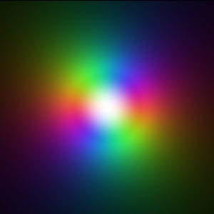
f(z) = Sqrt(z)
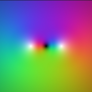
A dipole (+-)                       Two positive charges (++)
f(z) = 1/(z+1) - 1/(z-1)            f(z) = 1/(z+1) + 1/(z-1)